Tunneling Theory – Discretized Numerical Method
Tunneling Theory – Discretized Numerical Method. z. Long L = quantum wire short L = quantum point contact. (Must be obtained by a self consistent calculation for an accurate answer). Heterostructure with split gates- quantum wire/ quantum point contact. Plane waves in x direction.

Tunneling Theory – Discretized Numerical Method
E N D
Presentation Transcript
Tunneling Theory – Discretized Numerical Method
z Long L = quantum wire short L = quantum point contact (Must be obtained by a self consistent calculation for an accurate answer) Heterostructure with split gates- quantum wire/ quantum point contact Plane waves in x direction Confinement creates modes in y direction Total wave function is a linear combination over right and left traveling modes : fn(y) depend on V(y) A mode propagates if :
Conductance for an IDEAL quantum point contact or quantum wire at T= 0 K drain source Current flows from left 2DEG to right, due to difference in chemical potentials Current due to nth propagating mode: It can be shown for 1D subbands that : Since the velocities cancels out, the total conductance for M propagating modes is given by:
1 µm Conductance for REAL quantum point contact or quantum wire Gate voltage V reduces effective width - fewer modes, thus see a progression of steps QPC BJ van Wees et al Phys. Rev. Lett. 60, 848 (1988) Ideal formula generally not obeyed- imperfections such as impurities, boundary roughness or deliberately introduced structure cause waves to be only partially transmitted wire G Timp et al Nanostructure Physics and Fabrication, Academic Press, New York (1989)
A “quantum wire” with deliberately introduced structure- the quantum dot Cavity enclosed in both x and y directions- “artificial atom” Size of quantum dot typically studied is significantly smaller than the inelastic scattering length or mean free path- oscillations in G are almost exclusively due to the confinement Modes only partially transmitted in this case due to interference from multiple scattered waves inside the dot Ballistic quantum dots
To study these structures theoretically, a more general formula for conductance is required, to take into account partial transmission of modes If T(E) is the total transmission coefficient for all the modes then the current is given by: If Dm is small, then: The conductance then becomes The problem of calculating the conductance is one of finding the total transmission coefficient
Transfer-Scattering matrix formalism Case 1: 1D problem - transmission through a potential barrier II III I V=Vo V=0 V=0 x=0 x=b Plane wave with unit amplitude incident from left side only Boundary conditions: The reflection and transmission amplitudes Must solve for:
Wave function and its derivative must be continuous at the boundaries (a) (b) (c) More generally, one can write: Transfer matrix relating region I (left) with III (right) (c)
Put in boundary conditions: reflection coefficient transmission coefficient current conservation Alternate formulation- the scattering matrix Incoming waves outgoing waves
Case 2: 2D problem - infinite square well quantum wire with structure mode matching expansions w w2 I y=0 V=0 III II x=0 x=b
Evanescent modes Exponentially growing and decaying wave functions for n > M Generally, one can cut off number of evanescent modes in summations and still have answer converge. With cutoff, the matching problem now becomes a matrix problem that relates vectors of coefficients:
2D transmission problem - infinite square well quantum wire with structure y=0 Continuity at boundaries allows us to eliminate variables: Transfer matrix relating region I (left) with III (right)
One propagating mode Same equations as before, but with single coefficients replaced by matrices: Matrix elements of t Total transmission Transmission from mode m on left to mode n on right For square well model Result of a T-stub calculation with mode matching: Resonant tunneling peak Resonant reflection from a quasibound state
ntot should be large enough to include evanescent modes Exponentially growing and decaying wave functions in x direction. Generally, one can cut off number of evanescent modes in summations and still have answer converge. The transmission problem - waves of unit amplitude incident from left Matrix elements of transmission matrix Total transmission velocities = Transmission from mode m on left to mode n on right - sum over propagating modes ONLY
More complicated structures 1 2 3 4 5 6 7 8 Net transfer matrix is a product of the matrices for the individual sections Major problem- numerical instability due to the evanescent modes: terms overflow/underflow after a few matrix products are taken
Scattering matrix version: Incoming waves outgoing waves Relations between the scattering matrix and the transfer matrix: Note the presence of matrix/ matrix inverse products. The T’s contain many elements proportional to: due to the inclusion of the evanescent modes. These terms get cancelled out in the scattering matrix.
Solution- cascading scattering matrix Exploit cancellation of exponential factors in S matrix Need to find To solve problem Do so in an iterative manner
Split gate pattern eigenvalues eigenfunctions Realistic simulation of an experimentally studied quantum dot Measured conductance 2DEG The determine the confining dot potential from a numerical solution of the three-dimensional (3D) Poisson equation: • and the 1D Schrödinger equation: Step 1: • The Exchange and Correlation corrections to the ground state energy of the are included by using the Local Density Approximation.
V(x,y) is not a simple function • A magnetic field is applied When: Then the modes: can no longer be expressed as well characterized analytical functions Problems with simple mode matching: This is the case with the result of a realistic simulation For better flexibility and accuracy it is advantageous to do the problem on a discrete lattice. Still use modes, but determine them numerically, rather than using preset functions Confining potential has the form of a truncated parabolas
y x Calculate conductance using finite difference grid Wavefunction and potential defined on discrete grid points i,j j=M+1 transmitted waves incident waves reflected waves j=0 i=0 i=N i th slice in x direction - discrete problem involves translating from one slice to the next. Grid spacing: a<< lF
Obtaining transfer matrices from the discrete SE apply Dirichlet boundary conditions on upper and lower boundary: j=M+1 j=M Wave function on ith slice can be expressed as a vector Discrete SE now becomes a matrix equation relating the wavefunction on adjacent slices: j=1 j=0 (1b) i where:
(2) Is the transfer matrix relating adjacent slices where (1b) can be rewritten as: one obtains: Combining this with the trivial equation Modification for a perpendicular magnetic field (0,0,B) : B enters into phase factors important quantity: flux per unit cell
An aside – how the Peierl’s substitution appears in a tight-binding Hamiltonian magnetic field (Peierls substitution)
yields the modes on the left side of the system Solving the eigenvalue problem: Mode eigenvectors have the generic form: redundant There will be M modes that propagates to the right (+) with eigenvalues: propagating evanescent There will be M modes that propagates to the left (+) with eigenvalues: propagating evanescent defining and Complete matrix of eigenvectors:
Transfer matrix equation for translation across entire system Unit matrix waves incident from left have unit amplitude Transmission matrix reflection matrix Zero matrix no waves incident from right Converts back to mode basis Converts from mode basis to site basis In general, the velocities must be determined numerically Recall:
Variation on the cascading scattering matrix technique method Usuki et al. Phys. Rev. B 52, 8244 (1995) Boundary condition- waves of unit amplitude incident from right plays an analogous role to Dyson’s equation in Recursive Greens Function approach Iteration scheme for interior slices Final transmission matrix for entire structure is given by A similar iteration gives the reflection matrix
After the transmission problem has been solved, the wave function can be reconstructed It can be shown that: wave function on column N resulting from the kth mode One can then iterate backwardsthrough the structure: The electron density at each point is then given by:
u1(+) for B=0 T First propagating mode for an irregular potential u1(+) for B=0.7 T u1j Mode functions no longer simple sine functions confining potential 40 80 0 j general formula for velocity of mode m obtained by taking the expectation value of the velocity operator with respect to the basis vector.
Conduction band profile Ec 0.8 Energy of the ground subband 0.6 Conduction band [eV] 0.4 Vg= -1.0 V Vg= -0.9 V Vg= -0.7 V 0.2 Fermi level EF 0.0 z-axis [mm] -0.2 0.00 0.02 0.04 0.06 0.08 0.10 Example – Quantum Dot Conductance as a Function of Gate voltage Simulation gives comparable 2D electron density to that measured experimentally Potential felt by 2DEG- maximum of electron distribution ~7nm below interface Potential evolves smoothly- calculate a few as a function of Vg, and create the rest by interpolation
-0.897 V -0.923 V -0.951 V Same simulations also reveal that certain scars may RECUR as gate voltage is varied. The resulting periodicity agrees WELL with that of the conductance oscillations* Persistence of the scarring at zero magnetic field indicates its INTRINSIC nature The scarring is NOT induced by the application of the magnetic field Subtracting out a background that removes the underlying steps you get periodic fluctuations as a function of gate voltage. Theory and experiment agree very well
Magnetoconductance B field is perpendicular to plane of dot classically, the electron trajectories are bent by the Lorentz force Conductance as a function of magnetic field also shows fluctuations that are virtually periodic- why?
15.5 X Y E (meV) Y X 14.0 -0.25 0.25 B (T) The results of conductance calculations done win the presence of a field Corresponding wave functions: Wave function scarred by a diamond orbit. Arrows point to resonance lines along which the scar occurs Wave function that corresponds to a “bouncing ball” resonance Some individual conductance traces taken from the color plot: Lighter color = higher conductance
One what basis can one associate these wave functions with classical orbits? classical distribution shows similar pattern-trajectories bent by Lorentz force Wave function with “diamond” scar current amplitude shows circulation around the scar quantum “bouncer” classical “bouncer”
3.0 2.0 0.06 T 0.17 T SPECTRAL AMPLITUDE T=0.01 K 1.0 0.39 T 0.28 T 0.0 0 20 40 60 80 FREQUENCY (1/TESLA) Scarring periodicity and how it relates to experiment Recurring scars with period D B ~ 0.11 T, or 1/D B ~ 9 1/T Experimental trace for a ~0.3 mm dot Usually don’t see sharp resonances in experiment because of broadening effects (eg. finite temperature) major peak at ~9 1/T corresponds with scarring period Fourier transform However, periodic pattern still holds up even when broadening included to reduce sharpness The dominant frequency of the conductance fluctuations is given by the period of the scars
generalization: non-uniform grid vector form:
Generalized Peierls substitution Appropriate vector potential: for integration purposes, assume a linear variation of y between x slices: integrating for the inter-slice phase factors thus yields: Corresponding change to inter-slice matrices:
into this equation goes... hopping terms can no longer treated as simple scalars, matrix formulation becomes important tL,ihas similar diagonal form
Non-uniform mesh example B= 0 T model a QPC by keeping the number of mesh points in the y-direction fixed while reducing the lattice spacing B= +1 T y (mm) B= -1 T x (mm)
System with analogous physics: molecular wire problem can be expressed in terms of orbital hopping terms, ti,j , and site energies, Ui,j Can thus be modeled using However, depending on the problem, further generalization may be required need not be tridiagonal need not be diagonal • Such complications occur when... • bonding arrangement cannot be mapped onto a rectangular grid • orbitals on different sites overlap
Some useful references: D.Y.K. Ko and J.C. Inkson, Phys. Rev. B, 38, 9945 (1988). -Discusses the cascading scattering matrix method H. U., Baranger and A. D. Stone, Phys. Rev. B 40, 8169 (1989). -Discusses the velocity operator used to determine the mode velocity Karl-Fredrik Berggren and Zhen-li Ji, Phys. Rev. B, 43, 4760 (1991). -Discusses mode-matching T. Ando, Phys. Rev. B, 44, 8017 (1991). -Discusses the finite difference approach, then uses it to develop Recursive Green’s functions