Memory vs. Model-based Approaches
Memory vs. Model-based Approaches . SVD & MF Based on the Rajaraman and Ullman book and the RS Handbook. See the Adomavicius and Tuzhilin , TKDE 2005 paper for a quick & great overview of RS methodologies. . Basics . So far we discussed user-based and item-based CF.

Memory vs. Model-based Approaches
E N D
Presentation Transcript
Memory vs. Model-based Approaches SVD & MF Based on the Rajaraman and Ullman book and the RS Handbook. See the Adomaviciusand Tuzhilin, TKDE 2005 paper for a quick & great overview of RS methodologies.
Basics • So far we discussed user-based and item-based CF. • In both, we predict an unknown rating by taking some kind of aggregate of: ratings on the distinguished item by the distinguished user’s most similar neighbors (user-based) or ratings of the distinguished user on the distinguished item’s most similar neighbors (item-based). • Both based on a literal memory of past ratings: thus, memory-based. • Both look at closest neighbors: thus, neighborhood-based.
Model-based approaches • Build a model of each user’s behavior: what s/he looks for in an item. • Build a model of each item: what does it have to offer. • Problem: these “features” are not explicitly present. • Turn to latent features. • Matrix factorization: Approximate ratings matrix as a product of two low-rank matrices. • Dimensionality reduction. • Components of each user/item vector – latent factors/features.
serious Braveheart Amadeus The Color Purple Lethal Weapon Sense and Sensibility Ocean’s 11 Geared towards females Geared towards males Dave The Lion King Dumb and Dumber The Princess Diaries Independence Day Gus Stolen from: Bell, Koren, and Volinsky’s Netflix Prize talk. escapist
I T E M S U S E R S
MF (contd.) • computed to best fit known ratings. • Singular Value Decomposition (SVD) solves a related problem, but is undefined when the given matrix is incomplete (i.e., unknown entries). • If very few known ratings, risk of overfitting. • It’s instructive to recall how SVD works to better understand the foundations of MF.
SVD Recap • Given a matrix of rank , we can express it as • Orthogonal eigenvectors of • Orthogonal eigenvectors of • being the eigenvalues of or equivalently, the eigenvalues of [singular values.]
SVD Recap (contd.) • We can find a low-rank approximation using SVD framework. For a small rank zero out the smallest singular values. • Find • Notice, now we have of order of order of order and of order • This “reduced” form of SVD is what is used in many applications where data is large and computation is intensive. • Best possible rank--approximation under Frobenius norm of the error of approximation by any such matrix.
Returning to MF • Recall, in MF you factor a given ratings/utility matrix into • Caution: In the literature, you will sometimes encounter, the “transpose notation” -- • Problem: Find latent user and item vectors {and }: is minimized. • .
MF Usage • In practice, we minimize the error above over a training subset of known ratings and validate against the test subset. • Challenges in minimizing error: multiple local minima. Typically use gradient descent method. • Basic Idea: • Initialize some way. • Iteratively Update: where is used to control the “step size”. E.g., • Stop when the aggregate error squared (e.g., sum) is a set threshold.
Some Enhancements • Things are not quite perfect: risk of overfitting; solution – regularization. • Redefine the error for one entry as That is, • Discourages vectors with large magnitude since we minimize error; thus overcomes overfitting. • We manage to get with not too large entries while approximating
Enhancements • Modified update equations: • Try different initializations: e.g., random, all s, all s, all , where #non-blank entries of random perturbation to this setting, from different distributions, etc. Try different initializations and orders (see below) and pick the best local minimum.
Enhancements • Visit (i.e., update) elements of in row-major or column-major order and in round robin. • Or choose a random permutation of the entries and follow that order. • Pick the best “local minimum”. Sometimes, we pick the average of the values returned by each local minimum, to avoid overfitting. • Keep in mind, in practice, we don’t quite manage to find local minimum: we stop when the drop in error between successive rounds is below a threshold. • Other bells & whistles are possible: e.g., adding effects of user’s rating bias and item’s popularity bias; these parameters then included in the regularization.
Extensions • Location-aware: recommend items depending on where you are. • Time-aware: e.g., recommend fastfood restaurants for lunch on weekdays and formal/classy ones for dinner; recommend shows that are currently in town; recommend games during hockey season; … • Context-aware: e.g., recommend a movie depending on your current company.
What if feedback was implicit • More common than explicit feedback: • Not every customer will bother to rate/review. • Purchase history of products. • Browsing history or search queries. • Playcount in last.fm is a kind of implicit feedback. • Simple thumbs up/down for TV shows. Based on: Y.F. Hu, Y. Koren, and C. Volinsky, Collaborative Filtering for Implicit Feedback Datasets, Proc. IEEE Intl Conf. DataMining (ICDM 08), IEEE CS Press, 2008, pp. 263-272.
What is different about implicit feedback? • Just “adopt/no adopt” data inherently only gives positive feedback. • For all missing pairs, user may or may not be aware of the item: we know nothing about those cases. • Contrast: in explicit f/b, ratings do include negative f/b. However, even there, missing data doesn’t necessarily mean negative info. • Data may not be missing at random: question of what the user is aware of. • It’s in the missing part where we expect our negative signals. Cannot “ignore” missing data unlike with explicit f/b.
More Differences • Even the so-called positive cases are noisy. E.g., • Tune to a certain TV channel and talk to a friend the whole time. • Perhaps my experience after buying a smartphone was negative. • Perhaps I bought that watch as a gift. • No way of knowing! • Explicit f/b (rating) preference; implicit f/b confidence. E.g., • How often do I watch a series and for how long? • Playcount of songs on last.fm. • Evaluation metric – unclear; needs to account for availability and competition.
Basics • Natural to consider all missing values. (Why?) • Neighborhood-based methods face an issue: implicit f/b such as watching/listening frequency may vastly differ between users (unlike everyone rating on the same scale). • Rating biases exist but differences in watching/listening frequency can be much larger and can exacerbate the situation. • Complicates similarity calculation.
A Model • -- observations in the form of adoption or counts. Binarized to: if and otherwise. Think of as belief of user liking or not liking item. • We posit a confidence in our belief • ( found to work best by authors.) • min. confidence is 1 (no observations!). • Use MF as before with some important differences. • , where are -dimensional user and item latent vectors. How do we learn them?
A Model i.e., • Note, error being computed over all entries, including where no observations are available. The confidence can vary widely (see confidence expression). • obtained by cross-validation. • Mere error computation is prohibitive (unlike for explicit feedback) – significant challenge. (SGD won’t scale!) • Alternating Least Squares (which has been used in the ratings world as well) to the rescue! • ALS idea: Alternately treat the item factors or the user factors as fixed and try to minimize the error w.r.t. the other until “convergence”. error
In Implicit Feedback MF so far … • Observations (playcounts, adoption signals, etc.) lead to beliefs (which are binary) of user liking item, along with a confidencemore observationsmore confidence. • We want to predict missing along with corresponding confidences: i.e., currently our beliefs in these cases is “not like” and we’d like to revise them. • Unlike explicit f/b case, must treat all entries including missing ones (zero observations cases) – computing even the error of a given model is prohibitive! • Need to reassess the error, update user/item factors iteratively until convergence. scalability challenge unique to implicit f/b case.
ALS Details • Equating partial derivative of error w.r.t. to 0 and doing some elementary matrix calculus, and solving for we get , where the matrix with row being . Equiv., = the matrix whose column is . is and • Similarly, .
A Scalability Trick • Challenge: Speaking about users, must be computed for each of users. direct approach will take time! • Note: all diagonal elements of are • Consider only diagonal elements are non-zero, where = # elements user has “clicked”. • Write as Precompute in Time. Compute in time.
Scalability Story (contd.) • Overall work for one user Invert an matrix + its product with • Do right associative multiplication: has just elements, leveraging which we can do the above product in time. • Even assuming a naïve matrix inversion algorithm, total work for user can be done in time and for all users in time where = no. of non-blank entries in • Which is usually quite small. • Empirically, authors find acceptable. Essentially, linear running time: no. of alternations needed in practice is small (a few tens at most).
Recommendation Generation • user recommend the top- items with the highest • Worth experimenting with recommending items with the highest • where is the confidence in the prediction, not handled in the paper. • Analogy: score of a paper given by a reviewer & confidence of reviewer are both (to be) used in computing overall score! • One drawback: paper does not derive confidences for predictions! Scope for research.
What freedom do we have? • We could transform the observations into beliefs and confidences differently: e.g., use a threshold and use a smoother function for such as • We can still guarantee linear running time. Read paper for experimental study/evaluation.
Interesting side benefits • Potential use for explaining recommendation. • Potential for incremental computation? How similar are items and in ’s eyes.