Patch based Approaches
Patch based Approaches. A classification of multi-site scenarios. Metapopulation models. Most theoretical metapopulation models assume that all populations have identical extinction rates, and that they are all equi-distant from one another (e.g. Harrison and Quinn 1989)


Patch based Approaches
E N D
Presentation Transcript
Metapopulation models • Most theoretical metapopulation models assume that all populations have identical extinction rates, and that they are all equi-distant from one another (e.g. Harrison and Quinn 1989) • But these models are too far removed from realities of specific multi-site situations to be of practical use for particular species.
Incidence function models • Developed by Hanski (1991, 1994) • Sjögren-Gulve and Ray 1996, Moilanen 1999, 2000 and Kindvall 2000) Ilkka Hanski Atte Moilanen
The Incidence function model Use patterns of patch occupancy over time and space (“incidence’) to estimate: Ei, the probability of extinction for habitat patch i when it is occupied, and Ci, the probability that patch i becomes colonized when it is occupied Taking in account the patch’s habitat area, habitat quality, distance to other populations, and other potentially important characteristics
The Incidence function model • We start assuming specific function forms for the effects of the causal factors (patch area and quality, proximity of other populations, etc) on Ei and Ci.
Extinction e=1 x=0.5 A= area P(extinction ) in patch i Area
Colonization M= number of migrants y=1 P(colonization) in patch i Arriving migrants
The number of migrants • depends on: • The probability of other patches having extant populations, their population sizes (which is assumed to be proportional to the area of each patch), the rate at which dispersers leave the patch, and the distances from each other patch to focal patch i.
The number of migrants Mi= number of migrants β = per-unit-area migrant production rate A= patch i area Scaled by parameter b to allow for nonlinearity pj= 0 = empty and pj=1 if occupied α= scaling factor
A=10 A=20 Number of migrants (M) distance Number of migrants A= area
The incidence function model The probability that site i is occupied in any one site is predicted by in cases where rescue effects are thought to occur
The incidence function model • A snap-shot of the pattern of patch occupancy can be used to estimate the parameters governing Ci and Ei However, it means assuming that the occupancy patterns seen in the field are very near their equilibrium values
The incidence function model Where e’=ey’ and y’=y/β
Information needed • Mean population growth rate • Variance in population growth rate • Covariance in population growth rate • Probabilities of movement between populations • Estimates of density dependence
The California clapper rail Harding et al 2001
The California clapper rail 0.06*0.79*0.72=0.034 Harding et al. 2001
λMt 0 0 nM(t+1) nM(t) 0 λFt 0 nF(t+1) nF(t) 0 0 λLt nL(t+1) nL(t) The transition matrix • Determining counts at different sites =
nM(t+1) nM(t) nF(t+1) nF(t) nL(t+1) nL(t) The transition matrix • Determining counts at different sites (1-d)λMt da da = da (1-d)λFt da da da (1-d)λLt d=constant probability of an individual dispersing a=constant probability of an individual arriving
Effect of correlations With correlations Without correlations
Effect of levels of dispersal 20 % move 10 % move 5 % move none move
0 0 0 f4s4 s1 s2(1-g2) 0 0 0 s2g2 s3(1-g3) 0 0 0 s3g3 s4 The basic model Seeds Small juveniles Large juveniles Adults A=
0 0 0 0 0 0 0 0 0 0 0 0 0 0 0 0 0 0 0 0 0 0 0 0 0 0 0 f4as4a 0 0 0 f4c4c 0 0 0 f4bs4b 0 0 0 0 0 0 0 0 0 0 0 0 0 0 0 0 0 0 0 0 0 0 0 0 s1a s2a(1-g2a) 0 0 s1c s2c(1-g2c) 0 0 s1b s2b(1-g2b) 0 0 0 0 0 0 0 0 0 0 0 0 0 0 0 0 0 0 0 0 0 0 0 0 0 0 0 s2cg2c s3c(1-g3c) 0 0 s2bg2b s3b(1-g3b) 0 0 s2ag2a s3a(1-g3a) 0 0 0 0 0 0 0 0 0 0 0 0 0 0 0 0 0 0 0 0 0 0 0 0 0 0 0 s3ag3a s4a 0 0 s3bg3b s4b 0 0 s3cg3c s4c The multi-site model G=
0 0 0 f4bs4b(1-m-m) 0 0 0 f4as4a(1-m-m) 0 0 0 f4c4c (1-m-m) s1a s2a(1-g2a) 0 0 s1c s2c(1-g2c) 0 0 s1b s2b(1-g2b) 0 0 0 s2bg2b s3b(1-g3b) 0 0 s2cg2c s3c(1-g3c) 0 0 s2ag2a s3a(1-g3a) 0 0 0 s3ag3a s4a 0 0 s3bg3b s4b 0 0 s3cg3c s4c The multi-site model 0 0 0 f4as4a,mAB 0 0 0 f4as4a,mAC 0 0 0 0 0 0 0 0 0 0 0 0 0 0 0 0 0 0 0 0 0 0 0 0 0 0 0 f4as4a,mBA 0 0 0 f4as4a,mBC 0 0 0 0 0 0 0 0 G= 0 0 0 0 0 0 0 0 0 0 0 0 0 0 0 0 0 0 0 f4as4a,mcA 0 0 0 f4as4a,mCB 0 0 0 0 0 0 0 0 0 0 0 0 0 0 0 0 0 0 0 0 0 0 0 0