The Counterpropagation Network
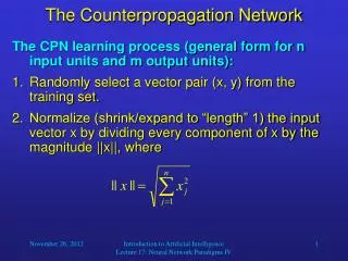
The Counterpropagation Network. The CPN learning process (general form for n input units and m output units): Randomly select a vector pair (x, y) from the training set. Normalize (shrink/expand to “length” 1) the input vector x by dividing every component of x by the magnitude ||x||, where.

The Counterpropagation Network
E N D
Presentation Transcript
The Counterpropagation Network • The CPN learning process (general form for n input units and m output units): • Randomly select a vector pair (x, y) from the training set. • Normalize (shrink/expand to “length” 1) the input vector x by dividing every component of x by the magnitude ||x||, where Introduction to Artificial Intelligence Lecture 17: Neural Network Paradigms IV
The Counterpropagation Network • Initialize the input neurons with the normalized vector and compute the activation of the linear hidden-layer units. • In the hidden (competitive) layer, determine the unit W with the largest activation (the winner). • Adjust the connection weights between W and all N input-layer units according to the formula: • Repeat steps 1 to 5 until all training patterns have been processed once. Introduction to Artificial Intelligence Lecture 17: Neural Network Paradigms IV
The Counterpropagation Network • Repeat step 6 until each input pattern is consistently associated with the same competitive unit. • Select the first vector pair in the training set (the current pattern). • Repeat steps 2 to 4 (normalization, competition) for the current pattern. • Adjust the connection weights between the winning hidden-layer unit and all M output layer units according to the equation: Introduction to Artificial Intelligence Lecture 17: Neural Network Paradigms IV
The Counterpropagation Network • Repeat steps 9 and 10 for each vector pair in the training set. • Repeat steps 8 through 11 until the difference between the desired and the actual output falls below an acceptable threshold. Introduction to Artificial Intelligence Lecture 17: Neural Network Paradigms IV
The Counterpropagation Network • Because the input is two-dimensional, each unit in the hidden layer has two weights (one for each input connection). • Therefore, input to the network as well as weights of hidden-layer units can be represented and visualized by two-dimensional vectors. • For the current network, all weights in the hidden layer can be completely described by three 2D vectors. Introduction to Artificial Intelligence Lecture 17: Neural Network Paradigms IV
The Counterpropagation Network • This diagram shows a sample state of the hidden layer and a sample input to the network: Introduction to Artificial Intelligence Lecture 17: Neural Network Paradigms IV
The Counterpropagation Network • In this example, hidden-layer neuron H2 wins and, according to the learning rule, is moved closer towards the current input vector. Introduction to Artificial Intelligence Lecture 17: Neural Network Paradigms IV
The Counterpropagation Network • After doing this through many epochs and slowly reducing the adaptation step size , each hidden-layer unit will win for a subset of inputs, and the angle of its weight vector will be in the center of gravity of the angles of these inputs. all input vectors in the training set Introduction to Artificial Intelligence Lecture 17: Neural Network Paradigms IV
The Counterpropagation Network • After the first phase of the training, each hidden-layer neuron is associated with a subset of input vectors. • The training process minimized the average angle difference between the weight vectors and their associated input vectors. • In the second phase of the training, we adjust the weights in the network’s output layer in such a way that, for any winning hidden-layer unit, the network’s output is as close as possible to the desired output for the winning unit’s associated input vectors. • The idea is that when we later use the network to compute functions, the output of the winning hidden-layer unit is 1, and the output of all other hidden-layer units is 0. Introduction to Artificial Intelligence Lecture 17: Neural Network Paradigms IV
network output if H3 wins network output if H1 wins network output if H2 wins The Counterpropagation Network • Because there are two output neurons, the weights in the output layer that receive input from the same hidden-layer unit can also be described by 2D vectors. These weight vectors are the only possible output vectors of our network. Introduction to Artificial Intelligence Lecture 17: Neural Network Paradigms IV
The Counterpropagation Network • For each input vector, the output-layer weights that are connected to the winning hidden-layer unit are made more similar to the desired output vector: Introduction to Artificial Intelligence Lecture 17: Neural Network Paradigms IV
The Counterpropagation Network • The training proceeds with decreasing step size , and after its termination, the weight vectors are in the center of gravity of their associated output vectors: Output associated with H1 H2 H3 Introduction to Artificial Intelligence Lecture 17: Neural Network Paradigms IV
The Counterpropagation Network • Notice: • In the first training phase, if a hidden-layer unit does not win for a long period of time, its weights should be set to random values to give that unit a chance to win subsequently. • There is no need for normalizing the training output vectors. • After the training has finished, the network maps the training vectors onto output vectors that are close to the desired ones. • The more hidden units, the better the mapping. • Thanks to the competitive neurons in the hidden layer, the linear neurons can realize nonlinear mappings. Introduction to Artificial Intelligence Lecture 17: Neural Network Paradigms IV