Understanding Network Layer Services & Routing: An In-depth Guide
Learn about network layer tasks like addressing, routing, and congestion control. Explore connectionless vs connection-oriented services and compare VC and DG routing. Discover routing algorithms like Dijkstra's and explore flow-based routing.

Understanding Network Layer Services & Routing: An In-depth Guide
E N D
Presentation Transcript
The Network Layer PC Router/Switch Server AP AP T T N N N N N DL DL DL DL DL PH PH PH PH PH
The Network Layer (cont’d) • Objective: getting packets from the source all the way to the destination of the subnet Subnet IMP IMP host host
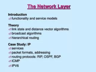
Main Tasks of the Network Layer • Providing services to the higher layer protocol • Addressing • Routing • Congestion Control • Internetworking • Accounting
Services Provided to the User Services perceived by the user applications can be categorized as: • Connectionless service • network is assumed to be unreliable • no connection setup prior to data exchange • applications need to handle packet ordering, error control, flow control, etc • for example, UDP Complexity is placed on the host.
Services Provided to the User (cont’d) • Connection-oriented Service • network should provide a reliable service • a connection is set up first and the two end points can negotiate about the parameters • packets are delivered in order and error-free. Flow control is automatic • for example, TCP Complexity is placed on the network.
Routing • Combinations of service and subnet structure Fig. 5-3, p. 346 • A major function of the network layer • Invoked at call set up time for the VC service • Invoked for every packet for the datagram service
Routing (cont’d) • Desired properties for routing • correctness • simplicity • robustness (to cope with topology and traffic changes) • stability (to converge to equilibrium) • optimality • fairness Fig. 5-4, p. 347
Routing (cont’d) • Nonadaptive (static) vs. adaptive routing • Optimality principle: If router J is on the optimal path from router I to router K, then the optimal path from J to K also falls along the same path. Fig. 5-5, p. 349
Virtual Circuit (VC) Routing • Connection-oriented routing in out Routing table at Node B a, 2 b, 5 Virtual channel ID g B a C b 5 2 Y A X F 6 D E
Datagram (DG) Routing • Connectionless routing dest out Routing table at Node B g Y Full destination address g B a C b Y 1 Y 3 A X F Y Y Y Y 3 2 1 Y 2 D E
Shortest Path Routing • Given: a graph of nodes (set N) and links (arcs) with associated arc weights (metrics), e.g. queue length, distance, delay and loss • For each origin-destination (O-D) pair find a path with the minimum total arc weights along the path • Centralized vs. distributed routing
Shortest Path Routing (cont’d) Routing table at Node A 5 • Each node computes the shortest paths to every other node in the network. • The metric of a link can be distance, delay, hop, bandwidth, or combinations of them. B C 2 4 3 3 dest next B B 2 A E F D C B D G E G 2 2 1 2 F G 4 G G G H H G
Shortest Path Routing (cont’d) • Dijkstra’s algorithm (to calculate a shortest path spanning tree rooted at node r) 0. S={r}, dist(i)=infinity for all i in N, dist(r)=0, l=r. 1. dist(i)=min{dist(i), dist(l)+cost(l,i)} for every neighbor of l where i is not in S. 2. Find among the nodes not in S a node with the minimum distance from r. Denote this node by l. 3. S=S unions {l}. 4. If S=N, stop; otherwise, go to Step 1.
Shortest Path Routing (cont’d) • Dijkstra’s algorithm (cont’d) Fig. 5-6, p. 349
Flooding • When a router receives a packet, the router duplicates the packet and broadcast it to all the links except the one from which the packet was received. • Flooding can be used to • discover all the routes between two points • exchange information network-wide
Flooding (cont’d) • Flooding will generate a vast number of duplicate packets. • Several ways to control flooding: • hop counter in each packet: packet is discarded when the counter is decremented to zero • maintain list of packets that have already been seen • selective flooding: only duplicate and send to those lines that could be right
Flow-based Routing • (Quasi-) static, capacitated and load sensitive • Given • topology • link capacities • traffic requirement (data rate for each O-D pair) • To determine: an optimal routing assignment • Objective: to optimize a certain performance measure, e.g. to minimize the average end-to-end packet delay • Subject to: multicommodity flow, nonnegativity and capacity constraints
Flow-based Routing (cont’d) • An example of evaluating the average end-to-end packet delay using M/M/1 queueing models Fig. 5-8, p. 354
Flow-based Routing (cont’d) • An example of evaluating the average end-to-end packet delay using M/M/1 queueing models (cont’d) Fig. 5-9, p. 355
Distance Vector Routing • Also called Bellman-Ford or RIP A dAX Routing table at Node S Distance Next Desti- nation dSA dBX dSB B X S X 120 A Y 100 C dCX dSC C Y • Each router keeps monitoring distances (current queue length) to its direct neighbors • Once every T sec it exchanges the (Destination, Distance) vector with all its neighbors • New distance from S to X via Node i = dsi + dix • Store the i that gives the minimum distance
Distance Vector Routing Example (¥, -) (¥, -) (11, C) (9, D) (9, D) Entry for destination F 7 2 (¥, -) (4, F) (4, F) (4, F) (4, F) B C 1 1 3 4 2 2 (¥, -) (¥, -) (6, C) (6, C) (6, C) 2 4 D (¥, -) (¥, -) (12, E) (12, E) (11, B) A F 1 (0, F) (0, F) (0, F) (0, F) (0, F) 6 5 3 3 7 E (¥, -) (7, F) (7, F) (7, F) (7, F) Note: At lease N updates are required to reach steady state, where N = network diameter
Count-to-Infinity Problem A A B B C C D D ¥ ¥ ¥ 1 ¥ ¥ 1 2 ¥ 1 2 3 1 2 3 3 2 3 3 4 3 5 4 5 A comes up A goes down ¥ ¥ ¥ One Solution -- Split Horizon algorithm: The distance to destination X is not reported to the neighbor which is the next hop for the packets destined to X
Ping-Pong Effect (D, 2, C) (D, 3, B) (D, 4, B) A (D, ¥) (D, 2) C D Suppose D goes down (D, 1, D) (D, ¥, -) (D, ¥, -) (D, 2) (D, ¥) B (D, 2, C) (D, 3, A) (D, 4 ,A) Packets for D will be bounced back-and-forth between A and B.
Link State Routing • Discovering the neighbors • a just booted router sends HELLO packet on each link it connects • its neighbors reply with their names • Measuring link delays • send ECHO packet to each neighbor and record how soon the reply comes back • OSPF, IS-IS are based on link state routing. Link state routing has five steps:
Link State Routing (cont’d) • Building link state packets every T seconds A 2 Seq # B C Age 4 1 3 B 4 E 5 A D 5 6 4 8 E F E Seq # Age A 5 C 1 F 8
Link State Routing (cont’d) • Distributing the link state packets by flooding • source increments the seq# for each new packet • when a router receives a packet, check its (source, seq#) • duplicate packet is discarded • new packet is broadcast to all the lines except the incoming one • age: decremented by each router. The packet is discarded when age goes to 0 • Computing the new routes • each node constructs the entire network topology, and then • computes the shortest paths to all possible destinations
Hierarchical Routing • The network is divided into hierarchies to reduce the size of the routing table Region 2 Region 1 Routing table at Node 1A 1B 1A Distance Next Dest 1C 1D 1B 60 1B 1C 80 1C 1D 110 1B 2 150 1B 3 180 1C 4 220 1C Region 3 Region 4
Hierarchical Routing (cont’d) • A router has one entry, in its routing table, for each router in the same region, and also one representation entry for each of other regions. • Example: For a subnet with 720 routers partitioned into 24 regions of 30 routers each, each router needs 53 entries (30 local + 23 remote). • For a subnet with n routers, the optimal number of hierarchical levels is ln(n) and the number of entries per router is eln(n).
Routing for Mobile Hosts • The mobile user first registers with the foreign agent, which then notifies the user’s home agent. 1. A packet is sent to the mobile host’s home address 4. Subsequent packets are tunneled to the foreign agent Home agent 3. Sender is notified of foreign agent’s address User’s home location Mobile user 2. Packet is tunneled to the foreign agent Foreign agent
Broadcast Routing • Possible methods: flooding, multi-destination routing, optimal sink tree, reverse path forwarding • Reverse path forwarding: approximate the optimal sink tree (router checks to see if the packet arrived on the line that is normally used to send packets to the source of the broadcast) I B • C • B • C • F H J N D • A • D • A • F • F • E • A D E K G O M O E • G • I • G • I • E C G D N K H • H • • N • J • L • N • J • L H B L • K • K • M • O • M • O L B
Multicast Routing • Multicast: sending a message to a group of nodes • Hosts may join or leave groups • Routers must know which of their hosts belong to which groups, and inform other routers A B C A B C D E Multicast router D E • MBone has been operational since 1992 to multicast live audio and video on the Internet
Multicast Spanning Tree 2 • Drawback: it scales poorly to large networks 1 1, 2 Source 2 1 1 2 2 1 1 1, 2 1, 2 Source Source 2 2 1 1 1 1 Spanning tree for Group 1 Spanning tree for Group 2
Congestion Control • Factors that cause congestion • insufficient buffer • slow CPU • low-bandwidth lines Perfect Maximum capacity Controlled Packets delivered Uncontrolled Deadlock Packets sent Need to upgrade both
Congestion Control (cont’d) • Main reason: Uncontrolled sharing of resources (buffer, bandwidth, etc.) D 10 kbps ALOHA, CSMA/CD X Throughput A B 100 kbps 10 kbps The A to B stream uses up most of the buffer at X 10 kbps Load C
Congestion Control (cont’d) • Congestion tends to feed upon itself Congestion backs up • Congestion control • make sure the network is able to carry the offered traffic • Flow control • make sure the sender does not overload the receiver in an point-to-point (or end-to-end) connection
Congestion Control (cont’d) • The flow control (sliding window protocol) at the data link layer does not prevent congestion at the network layer D F 10 kbps 10 kbps X A B 10 kbps 10 kbps Need a way to slow down the source, i.e., change the window size dynamically 10 kbps 10 kbps E C
Congestion Control Principles • Preventive control: take actions way before congestion ever happens • action at source • action at destination • Corrective control: detect congestion via feedback and take corrective actions • 1. Detect 2. Inform source 3. Action • Explicit feedback • Implicit feedback • Action: increase capacity, or decrease load
Traffic Shaping • A preventive control scheme • Force the source to transmit packets in a more predictable way (different from sliding window control) • Source and the network agree on a traffic pattern during VC setup • Algorithms • Leaky Bucket Algorithm • Token Bucket Algorithm
The Leaky Bucket Algorithm • Each host is connected to a leaky bucket interface • The bucket allows one packet to pass every DT sec • If a packet arrives and the bucket is full, the packet is discarded • The output rate is very rigid Host Unregulated flow Capacity = C Leaky Bucket control (just a finite buffer) Regulated flow Network
The Token Bucket Algorithm • A token is generated every DT sec • The bucket can hold at most n tokens • Each packet must capture a token before it can be transmitted • Host negotiates with the network on • n, DT, max packet size, max transmission rate Before After Host Host Token Bucket Network Network
Admission Control • When congestion occurs, allow no new VC (A to B) setup, or route new VC (A to C) around congested area • Works on VC only B Congestion A C
Choke Packets Router • A choke packet is sent to the source when the output line is congested • The source reduces its traffic to B by certain percentage (e.g., 50 % each time) • A variation is to have the choke packet take effect at every hop it passes through Choke packet Reduce traffic to B A to B A Host A B
Load Shedding • A router drops packets when it is congested • Which packets to drop depends on applications, e.g., • for file transfer: dropping young packet is better • for real time application: dropping old packet is better • Applications mark their packets to different priority classes • low priority to be dropped first at congestion • need policy to enforce this
Congestion Control for Multicasting • RSVP - Resource reSerVation Protocol • The receiver initiates the bandwidth reservation before receiving traffic 1 2 1 2 1 2 A B C A B C A B C Bandwidth reserved for source 2 Bandwidth reserved for source 1 D E F D E F D E F G H I G H I G H I J K L J K L J K L 3 4 5 3 4 5 3 4 5
Internetworking • Different networks exist today: TCP/IP, SNA, DECnet, SPX/IPX, AppleTalk, ATM, Wireless • Networks differ at protocols, VC/DG, addressing, packet size, QoS, etc. Multiprotocol Router Token Ring SNA IBM mainframe X.25 WAN Ethernet Ethernet Hub
Interconnecting Devices • Layer 1: repeater ---- copy bit by bit • Layer 2: bridge (hub, Ethernet switch) • store and forward frames • interconnect multiple LANs • Layer 3: Multiprotocol routers • store and forward packets • interconnect different types of networks (IP, IPX,..) • Layer 4: Transport gateway • e.g., conversion between TCP and ATM connections • Layer 7: Application gateway • e.g., conversion between different email packages
Full Gateway and Half Gateway Packet of Net 1 Packet of Net 2 G Net 1 Net 2 Full gateway Neutral Packet Net 2 Net 1 Half gateway