Network Layer Functionality and Service Models
Explore the network layer's key concepts, including routing algorithms, broadcast algorithms, and router functionalities. Learn about IP and ATM services, packet formats, and addressing. Discover the differences between Virtual Circuit and datagram services. Understand the importance of routing tables and the theoretical basis of routing algorithms. Dive into centralized vs. decentralized routing and static vs. adaptive routing approaches.

Network Layer Functionality and Service Models
E N D
Presentation Transcript
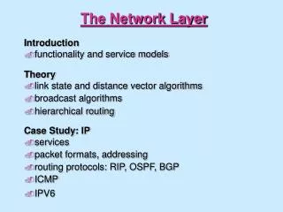
The Network Layer Introduction • functionality and service models Theory • link state and distance vector algorithms • broadcast algorithms • hierarchical routing
The Network Layer (cont) Case Study: IP • services • packet formats, addressing • routing protocols: RIP, OSPF, BGP • ICMP • IPV6 Case Study: ATM • services • cell formats • VP's and VC's
The Network Layer (cont) Routers and Switches how they work Readings • Tannenbaum: 5.1, 5.2, 5.4-5.7 • Ross, Kurose: 4.1-4.4, 4.6,4.7
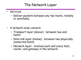
Network Layer: Introduction Network layer:a network-wide concern • transport layer: between two hosts • data link layer: between two physically connected hosts, routers • network layer: involves each and every router, host, gateway in the network
Network Layer Service: Virtual Circuit Virtual: looks like a circuit but isn't • generally associated with connection-oriented service • all packets within connection follow same route
At connection establishment time: • connection setup packet flows from sender to receiver • routing tables updated at intermediate nodes to reflect new VC • key issue: per-connection state at router • fits well with QoS guarantees: reserve resources and/or accept/reject call based on resources at this router Analogy: telephone network
Network Layer Service: datagrams • no notion of connection in network layer • no routes set up at connection establishment time - each packet in "connection" may follow different path • no guarantee of reliable, or in-order delivery • advantages: • no connection state in routers • robust with respect to link failures • recovery at end-systems (transport level)
Burning question: to VC or not to VC? Answer: support both, offering different service models: • best effort service: datagrams • service with performance guarantees: QOS
The routing function A network-layer packet contains: • transport layer packet (port, seq, ack, data, checksum, etc) • addressing info (e.g., source, dest. address or VC identifier) • other fields (e.g., version, length, time-to-live) Router/switch actions simple on packet receipt: • look up packet identifier (dest. address or VC id) in routing table and forward on appropriate out-going link (or upwards if at destination)
Routing Table: issues Key question: how are routing tables determined/updated? • whodetermines table entries? • what info used in determining table entries? • when do routing table entries change? • where is routing info stored? • how to control table size? • whyare routing tables determined a particular way. What is the theoretical basis? Answer these and we are done!
Routing issues: • scalability: must be able to support large numbers of hosts, routers, networks • adapt to changes in topology or significant changes in traffic, quickly and efficiently • self-healing: little or not human intervention • route selection may depend on different criteria • performance: "choose route with smallest delay" • policy: "choose a route that doesn't cross a government network" (equivalently: "let no non-government traffic cross this network")
Classification of Routing Algorithms Centralized versus decentralized • centralized: central site computes and distributed routes (equivalently: information for computing routes known globally, each router makes same computation) • decentralized: each router sees only local information (itself and physically-connected neighbors) and computes routes on this basis • pros and cons?
Classification (cont) Static versus adaptive • static: routing tables change very slowly, often in response to human intervention • dynamic: routing tables change as network traffic or topology change • pros and cons? Two basic approaches adopted in practice: • link-state routing: centralized, dynamic (periodically run) • distance vector: distributed, dynamic (in direct response to changes)
Link-state routing • each node knows network topology and cost of each link • quasi-centralized: each router periodically broadcasts costs of attached links • cost may reflect • queueing delay on link • link bandwidth • all links with equal cost: shortest path routes • used in Internet OSPF, ISO IS-IS, DECnet, "new" (1980) ARPAnet routing algorithm Goal: find least cost path from one node (source) to all other nodes • Dijkstra's shortest path algorithm
Dijkstra's Shortest Path Algorithm: Definitions Define: c(i,j): cost of link from i-to-j. c(i,j) = infty if i,j not directly connected. We will assume c(i,j) equals c(j,i) but not always true in practice D(v): cost of currently known least cost path from source, A, to node v. p(v): previous node (neighbor of v) along current shortest path from source to v N: set of nodes whose shortest path from A is definitively known Iterative: after k iterations, know paths to k "closest" (path cost) to A
Dijkstra's algorithm: Statement Initialization: N = {A} for all nodes v if v adjacent to A then D(v) = c(A,v) else D(v) = infty Loop: find w not in N such that D(w) is a minimum add w to N update D(v) for all v not in N: D(v) <- min( D(v), D(w) + c(w,v) ) /* new cost to v is either old cost to v or known shortest path cost to w plus cost from w to v */ until all nodes in N
example: in step 1: D(C) = D(D)+c(D,C) 1 + 3 • for each column, last entry gives immediate neighbor on least cost path to/from A, and cost to that node • worst case running time: O(N^2)
Distance vector routing Asynchronous, iterative, distributed computation: • much more fun! • at each step: • receive info from neighbor or notice change in local link cost • compute • possibly send new info to adjacent neighbors Computation/communication between network layer entities!
cost to dest. via 1 DE() A B D A 1 14 5 B 7 8 5 C 6 9 4 D 4 11 2 B C 7 8 2 A destination 1 E D 2 Distance table: • per-node table recording cost to all other nodes via each of its neighbors • DE(A,B) gives minimum cost from E to A given that first node on path is B • DE(A,B) = c(E,B) + min DB(A,*) • minDE(A,*) gives E's minimum cost to A • routing table derived from distance table • example: DE(A,B) = 14 (note: not 15!) • example: DE(C,D) = 4, DE(C,A) = 6
Distance vector algorithm • based on Bellman-Ford algorithm • used in many routing protocols: Internet BGP, ISO IDRP, Novell IPX, original ARPAnet Algorithm (at node X): Initialization: for all adjacent nodes v: D(*,v) = infty D(v,v) = c(X,v) send shortest path cost to each destination to neighbors Loop: execute distributed topology update algorithm forever
Update Algorithm at Node X: 1. wait (until I see a link cost change to neighbor Y or until receive update from neighbor W) 2. if (c(X,Y) changes by delta) { /* change my cost to my neighbor Y */ change all column-Y entries in distance table by delta if this changes my least cost path to Z send update wrt Z, DX(Z,*) , to all neighbors } 3. if (update received from W wrt Z) { /* shortest path from W to some Z has changed */ DX(Z,W) = c(X,W) + DW(Z,*) } if this changes my least cost path to Z send update wrt Z, DX(Z,*) , to all neighbors
Distance Vector Routing: Example Y 1 2 X Z 7
DX Y Z Y Z DX Y Z Y Z DX Y Z Y2 infty Z infty 7 DY X Z X Z DY X Z X Z DY X Z X 2 infty Z infty 1 DZ X Y X Y DZ X Y X Y DZ X Y X7 infty Y infty 1
Distance Vector Routing: Recovery from Link Failure • if link XY fails, set c(X,Y) to infty and run topology update algorithm • example (next page) • good news travels fast, bad news travels slow • looping: • inconsistent routing tables: to get to A, D routes through E, but E routes through D • loops eventually disappear (after enough iterations) • loops result in performance degradation, out-of-order delivery
Distance Vector Routing: Solving the Looping Problem Count to infinity problem: loops will exist in tables until table values "count up" to cost of alternate route Split Horizon Algorithm: • rule: if A routes traffic to Z via B then A tells B its distance to Z is infinity • example: B will never route its traffic to Z via A • does not solve the count to infinity problem (why)? A B Z
More problems: Oscillations A reasonable scenario • cost of link depends on amount of traffic carried • nodes exchange link costs every T • suppose: • A is destination for all traffic • B,D send 1 unit of traffic to A • C sends e units of traffic (e<<1) to A Entire network may "oscillate" Possible solutions: • avoid periodic exchange (randomization) • don't let link costs be increasing functions of load
Comparison of LS and DV algorithms Message complexity: • "LS is better": DV requires iteration with msg exchange at each iteration • "DV is better": if link changes don't affect shortest cost path, no msg exchange Robustness: what happens if router fails, misbehaves or is sabotaged? LS could : • report incorrect distance to connected neighbors • corrupt/lose any LS broadcast msgs passing through • report incorrect neighbor DV could: • advertise incorrect shortest path costs to any/all destinations (caused ARPAnet crash: "I have zero cost to everyone")
Comparison of LS and DV (cont) Speed of convergence DV: • may iterate many times while converging • loops, count-to-infinity, oscillations • cannot propagate new info until recomputes its own routes LS: • requires 1 broadcast per node per recomputation • can suffer from oscillations both have strengths and weakness • one or the other used in almost every network
2nd Try (at LS Broadcast Distribution) Each router puts a sequence number on its LSP's • upon receiving LSP(R) from R if (seq # > seq # of stored copy ) of LSP(R) then store LSP(R), update LS info for R, and flood LSP(R) else ignore duplicate How can this protocol fail?