The Network Layer
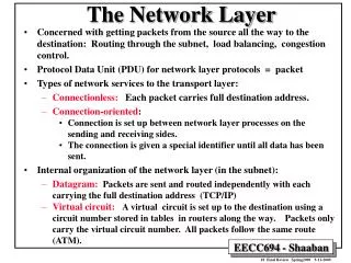
The Network Layer. Chapter 5. Routing Algorithms. Routing : Determines the path of a message from source to destination. Path is indirect (not broadcast network, ring, fully meshed network). Goals : Low transfer time: Few nodes along path Lowly utilized links/nodes


The Network Layer
E N D
Presentation Transcript
The Network Layer Chapter 5
Routing Algorithms • Routing: • Determines the path of a message from source to destination. • Path is indirect (not broadcast network, ring, fully meshed network). • Goals: • Low transfer time: • Few nodes along path • Lowly utilized links/nodes • Preferably links of high throughput • Even distribution of utilization if alternative paths exist • Adaptability to changes: • Load change • Crashes, repair • Network configuration (e.g. mobile network) • Simple, fair, robust algorithms with low information need
Routing Algorithms • Characteristics: • Exchanged Information: About nodes, links, transfer time, throughput, optimal routes, … • Cost function for optimality: Dependent on nodes, links, waiting time, … • Non-adaptive(or static) algorithm: Does not consider changes of load/availability • Adaptive (or dynamic) algorithm : Considers changes of load/availability • Centralized algorithm: Some node(s) run(s) the algorithm • Decentralized algorithm: Isolated/collective (distributed) • Restart of algorithm: Periodically/event-driven
Routing Algorithms Routing Non-adaptive Adaptive Centralized (or offline complete information) Isolated Decentralized Centralized Collective Periodic Isolated Event-driven (or periodic) Periodic Event-driven Routing Center Link State Routing Hot Potato Fixed routing tables Multi-path routing Distance Vector Routing Flooding In practice: Hierarchical routing e.g. non-adaptive centralized at country level and beneath another algorithm
Shortest Path Routing (Dijkstra Algorithm) Source: (A, 0 , -1) 2 6 (G, 5 , E) (G, 6 , A) (G, ¥ , -1) (G, 5 , E) (B, ¥ , -1) (B, 2 , A) (B, 2 , A) 1 2 (E, ¥ , -1) (E, 4, B) (E, 4, B) 4 7 2 (F, 6 , E) (F, ¥ , -1) (F, 6 , E) 3 2 (C, 9 , B) (C, ¥ , -1) (C, 9 , F) (C, 9 , F) (H, 9 , G) (H, ¥ , -1) (H, 8 , F) (H, 8 , F) 2 3 • Input: Network (of routers) with link weights. . • Output: shortest path between Source and Destination • Initialization: • Permanent nodes/tentative nodes • Steps: • Let X be the last permanent node • For allY in neighbor(X) If XY yields “better” path from Source to Ythen Update Y.Opt and Y.P • Find the tentative node Min with minimum Opt value • Set X to Min • If X = Destinationthen Stop • Else Goto first Step • Print path backwards using the P values • O(n2) algorithm Destination: (D, 10 , H) (D, 10 , H) (D, ¥ , -1) Data structure: (N: node, Opt: optimal distance to source , P: previous optimal node)
Routing Algorithms • Fixed Routing Tables: • After each network reconfiguration/change all routing tables are centrally or offline computed and sent to all nodes • Advantage: Optimal routing tables, network is not used for routing traffice • Disadvantage: Not robust against crashes or load changes • Rather acceptable in the version of multi-path routing: • For each packet a random number in [0, 1] is generated, which is used to select the neighbor to which the pack is sent, • Example (routing table in node Z): Target Neighbor X Neighbor Y A [0, 70%[ [70%, 1[ B [0, 60%[ [60%, 1[ • Alternatives paths are used for: • Dividing traffic (no probabilities): e.g. even utilization, divide depending on packet type (e.g. file transfer uses satellite, video uses ATM) • Fault tolerance: crash of neighbor or its link means the use of another (good if alternative paths are disjoint) • Multi-path routing is a general method not dependent on fixed routing tables
Routing Algorithms • Flooding: • Simple non-adaptive, isolated, non-informed algorithm • Each router forwards each packet to all its neighbors (except source neighbor) • To avoid packets circulating forever: • A hop counter is initialized by the sender to the maximum path length (in hops) and is decremented in each router. Any packet is destroyed, if its hop counter reaches 0. • A time stamp is initialized by the sender to the expected transfer time of the packet. Any packet is destroyed, if its delay is greater than its time stamp. • Each router remembers (using a per source sequence number) which packets have been received before, and destroys duplicates • Flooding has the advantage that it finds the shortest path to the destination, however, the search lasts a long time (since network is full). • More important: If there is a path, then flooding will find it. • In practice good if: • Extreme fault tolerance is needed (e.g. military area) • Topology is highly variable (e.g. wireless networks) • For initialization of routing tables • For broadcast (e.g. of time, updates)
Routing Algorithms • Hot Potato: • Fully isolated • In each router, the packet is forwarded along the link with the shortest queue . (router tries to get rid of packet as fast as possible – hot potato) • Not reliable, packet does not always reach destination • Distance Vector Routing: • Isolated with some information from neighbors • Bad but historically interesting algorithm (old ARPA routing) • Each router computes for each destination the optimal neighbor using periodically exchanged messages among neighbors. Exchanged information about ALL nodes but among neighbors ONLY • Problems: • High exchanged information volume • Information disseminates slowly in the network • Count-to-infinity problem (see below)
Routing Algorithms • Example for Distance Vector Routing: • Distances: (A, J) = 8, (I, J) = 10, (K, J) = 6, (H, J) = 12 • Old routing tables are not used (a) A subnet. (b) Input from A, I, H, K, and the new routing table for J.
Routing Algorithms 3 because C says 2 (+1) 4 because C’s neighbors are 3 (+1) rows Means router thinks that A is down (¥) rows: number of exchanged messages until all realize that A is down. rows should be bounded up by e.g. maximum path length in the network +1 • Distance Vector Routing: Count-to-Infinity Problem • Good news propagate fast • Bad news propagate very slowly • Example: • Good news: A is up (and was down): propagation speed 1 hop / period • Bad news: A is down (and was up): very slow propagation
Routing Algorithms • Link State Routing: • Collective dynamic routing algorithm • New ARPA routing algorithm • Well-used in practice • Each router computes for each destination the optimal neighbor using periodically/event-driven exchanged messages among all routers. Exchanged information about neighbors ONLY but among ALL routers • Each router must do the following: • Discover its neighbors, learn their network address. • Measure the delay or cost to each of its neighbors. • Construct a packet telling all it has just learned. • Send this packet to all other routers. • Compute the shortest path to every other router.
Routing Algorithms • Example for Link State Routing: • Packet format e.g. (Source router, Sequence number, Age, Data about neighbors) • Subnet. (b) Packets exchanged between routers. • Distributing Link State Packets: • Flooding • Duplicates detected using sequence numbers • Age field is used to invalidate information after some time (e.g. if source router X is down, age will become eventually 0 and entry of X in other routers is deleted) • Computing New Routes: Based on Dijkstra algorithm
Routing for Mobile Hosts • Mobile Hosts: • Migratory host: stationary ones that move from time to time (e.g. plug in in another LAN) • Roaming host: able to maintain connections while moving (e.g. laptops in a wireless LAN) MH HA FA A WAN to which LANs, MANs, and wireless cells are attached. • Registration with foreign agent (if new host enters its domain): • Periodically: FA all (in LAN):“I am here” or MH all: “Is there a FA” (after migration) • MH FA: Home address (HAddr), current layer-2 address (CAddr), Security data (SData) • FA HA: “one of your MH is here”, FA address, Sdata (to convince HA that FA is not lying) • HA FA: “Ok” if Sdata acceptable “No” if not • FA MH: “You are (not) registered” (FA remembers Caddr of MH in a table)
Routing for Mobile Hosts • A sender connecting to a mobile host: • Sender HA: packet1 (HA intercepts any packet destined to MH) • HA FA: [header1, packet1] (Tunneling: packet1 is in payload of a new packet!) • HA Sender: “Please tunnel subsequent packets to FA” • Sender FA: [header2, packet2], … Sender Home Agent Foreign Agent Packet routing for mobile users.
Routing in Ad Hoc Networks • Unlike routing for mobile hosts, the routing in ad hoc networks does not assume that the routers are fixed (in the WAN). • Everything can move (hosts & routers); in other words: every node is router (and host) • Example for mobile routers: • Military vehicles on battle field (no infrastructure) • A fleet of ships at sea (all moving all the time) • Emergency works at earthquake (infrastructure destroyed) • A gathering of people with notebook computers • Traditional routing algorithms cannot be applied, since: • No fixed topology: No fixed and no known neighbors • No fixed mapping network address (e.g. IP address) to location • … • AODV (Ad hoc On-demand Distance Vector) routing protocol: • Main idea (see textbook for details): • A sender that does not know how to reach a destination generates a ROUTE REQUEST packet that is broadcast hop by hop in the network until it reaches the destination or a node that knows how to get to destination. Each intermediate node memorizes where the request came from (to build the backward path). • Destination (or intermediate node) replies by ROUTE REPLY packet that goes back to the sender through the memorized backward path.
Routing in Ad Hoc Networks • A wants to send to I: • (a) A broadcasts ROUTE REQUEST (only B and D are in the range of A's broadcast). • (b) B and D receive packet; since they do not know how to get to I, they further broadcast the packet and • memorize how to get to A (backward arrow). • (c) New receivers of packet are C, F, and G, and they broadcast the packet further. • (d) Among the new receivers is I, the destination, thus I sends a unicast ROUTE REPLY to G. • Each node on the reverse path updates its tables and unicasts packet further in direction of • source.
Routing in Ad Hoc Networks • Failure (and out of range) detection: • To cope with nodes that fail or go out of the range of their neighbors the protocol includes the • exchange of periodic packets. • Consider node D if G goes down: • D detects failure because G does not react. • For each destination, D maintains in a routing table the set of predecessors (active neighbors) that recently have had traffic with that destination (here e.g. I has been recently destination for traffic from predecessors A, B using successor G) • D finds out that G is used for traffic destined to {E, G, I} and this traffic comes from {A, B}. Thus, D sends a packet to A and B saying that G is no longer reachable (through D). (a) D's routing table before G goes down. (b) The graph after G has gone down.
Routing in Peer-to-Peer Networks Java1.3 Search Java1.4 A Logo3.4 G Zip1.0 Acrobat 1.4 B Java1.4 GameA F Zip2.0 Acrobat 1.4 VideoX C E Song2 VideoY D Acrobat 2.0 Song1 • Users (or nodes) in a P2P Network: • Are symmetric (no hierarchy or central control). • Do not know each other. • Want to share resources (public domain programs, videos, music, …). • Know names of resources (e.g. zipX.Y). • Do not know where a resource of specific name is stored. • Their number is large if not very large ( e.g. >10 millions). • Example (see figure): • Naive solution: • Each node has a routing table that includes • addresses of all nodes in the network. • Node B asks then all nodes sequentially. • Problems: • Search is linear (inefficient) • Routing table too large • Violation of 2nd requirement (of above)
Routing in Peer-to-Peer Networks • Routing Protocol in Chord: • Let n be the number of nodes in the network. • Each node address (e.g. IP address) is hashed using SHA-1 algorithm in order to get an m-bit node ID (i.e. node ID = hash(IP address)) • Each resource name is also hashed in the same manner in order to get a m-bit key (i.e. key = hash(resource_name)) • The 2m node IDs arranged in ascending order in a circle (m=160 in current implementation) • Node ID name space = key name space (name both NS e.g. NS = {0, …, 2m –1}) • Since n << 2m the node ID space includes (many) IDs without actual nodes assigned to them. • Define the total function successor: NS NS, where: • successor(x) = ID of the first actual node following x (in the circle) • and the partial function IP: NS NS of IP, where: • IP(x) = IP address of x if x corresponds to an actual node, and undefined otherwise • Insertion of a new resource with name name at node x: • Store (name, IP(x)) in node with address IP(successor(hash(name))) • Search of resource with name name from node y: • Get (name, IP(x)) from node with address IP(successor(hash(name))) • Contact x using IP(x) to get the resource with name name • Problem: How to find IP(x)? • Each node maintains a (small) routing table (called finger table in Chord).
Routing in Peer-to-Peer Networks 1) Finger table FT at node x: FT[i] = (id[i], ip[i] ), where: id[i] = x + 2i (mod 2m) and ip[i] = IP(successor(id[i])) and 0 <= i < m 2) Also held by x: (successor(x), IP(successor(x))) 3) FT size small e.g. m=160 (or log(n)) 4) IDs in FT increase exponentially, hence search is O(log(n)) 5) Examples for search at node 1: a) key=3: since 1 < 3 < successor(1)=4, node 1 contacts IP(4) directly. b) key=14: 1 gets the closest predecessor of 14 from FT (9) and asks IP(successor(9)) = IP(12) to search further. Node 12 sees that 12 < 14 < successor(12)=15 and returns IP(15) c) key=16: 1 asks 12, 12 asks 15, and node 15 returns IP(20), since 15 < 16 < 20 (a) m = 32 node identifiers arranged in a circle (shaded ones correspond to actual machines) (b) Examples of the finger tables.
Congestion • Congestion (traffic jam) occurs because: • Queues build-ups in links (e.g. bridges) and routers. • Loss (destruction) of packets because of finite buffers for queues • even with infinite buffers problem still existent since packet will time out and will be resent • Slow processors in routers. • Low-bandwidth lines (connected to higher ones) • Problem is very complex because of different factors • Congestion control vs flow control: • Congestion control is a global issue that concerns measures controlling end systems, routers, and links in the network with the aim of making the network able to carry the offered traffic. • Flow control operates only locally between a pair of (adjacent) sender and receiver and tries to protect slow receivers from being overwhelmed with messages. • Principles of congestion control: • Open-loop control: constructively avoid congestion by good design without relying on network state • Closed-loop control: • Monitoring network state (e.g. queue length, packet transfer times, lost packets, ..) • Passing information to places where actions may be taken (e.g. choke packets to sources) • Adjusting system to end congestion (e.g. reduce sending rate of host)
Congestion (e.g. because of finite buffers, packet loss, congestion signals) When too much traffic is offered, congestion sets in and performance degrades sharply.
Congestion Control in Virtual-Circuit Subnets • Admission control: • If network congested, reject new connection requests until problem is resolved. • Avoid congested areas: • Connection from A to B normally goes through congested areas but routers decide for another • (longer but congestion-free) path. • Service level agreement (SLA): • Sender has a “contract” with network, which specifies traffic shape, volume etc. Network reserves • resources for sending host (e.g. at connection time) to avoid congestion. • tends to waste resources (and not to mention delay because of setup time) (a) A congested subnet. (b) A redrawn subnet, eliminates congestion and a virtual circuit from A to B.
Congestion Control in Datagram Subnets • Warning bit in packet header: • Routers should be able to detect congestion on their output links • If e.g. output link utilization is above a threshold, router sets a warning bit in header. • Receiver host (on transport layer) adds this bit to the ACK (going back to sender). • Sender monitors amount of ACKs (per time unit) that have the warning bit set. • Sender keeps decreasing its rate until the monitored amount decreases (no router in trouble). • Only then sender is allowed to increase traffic rate again. • used e.g. in Frame Relay • Router-to-Sender choke packets: • Idea: • If in trouble, a router contacts sender directly (unlike above, where traffic goes first to receiver) • If router detects congestion, it sends a choke packet to sender. • Choke packet: Has a bit set (to avoid generating more choke packets on the way to sender), • and it includes the destination (so that sender can identify the meant data stream). • Sender then reduces its traffic to specified destination by a fixed amount (e.g. 10%) • Sender ignores choke packets for that destination for a specified time (e.g. 60 sec) • After time has expired, sender waits another time interval, if no choke packet arrives, sender • increases its traffic, if some come sender reduces its traffic further.
Congestion Control in Datagram Subnets • Problem with Router-to-Sender choke • packets in high-bandwidth networks (see figure (a)): • Router (D) may be far away from sender (A) • (e.g. Toronto to Calgary) • Reaction is too slow • Example: Choke packet needs 30 ms to arrive to sender. At a rate of 155 Mbps, ca. 4.6 Mb have been sent in these 30 ms. Even if sender immediately shuts down, network must deal with the poured 4.6 Mb! • Hop-by-hop choke packets (see figure (b)): • Idea: • Immediate effect of choke packet on each hop it • passes through on its way to the sender. • +: better relief at congestion points (locally) • - : More congestion in routers upstream for a • while
Load Shedding • If overwhelmed, routers start to throw packets away (a nicer word: load shedding) • Policies of packet destruction: • Random: Select a packet at random • Milk: “New better than old” • e.g. in a multimedia stream, it is better to discard an older packet and let a newer one live further. • Wine: “Old better than new” • e.g. in file transfer, discarding an older packet may mean its retransmission later. Thus, it is better to discard a newer one. • Priority: Senders assign packets priorities, which are used by router to conduct discard policy. • RED (Random Early Detection): • Preventive method: Start discarding packets before congestion really happens. • Packet selection (for discard) is done randomly • No choke packet back to sender, but rather sender (transport layer) will time out (waiting • for ACK from receiver) and will slow down and resend packet again. • Main assumption: timeout = packet loss (!= packet received incorrectly) • Ok for (reliable) fixed networks, but not suitable for wireless networks (which are in general less reliable)
Jitter Control • Jitter: Variance of delay. • Very important for multimedia applications. • Example: • Video on Demand (VoD) • Buffering is done at the receiver to cope with the jitter problem. • However, for interactive real-time applications like video conferencing, routers are responsible for buffering: • If packet behind of schedule, router forwards it quickly. • If packet ahead of schedule, router buffers it for a while, and forwards it later.
The Internet The Internet is an interconnected collection of many networks.
The IP Protocol VER: version e.g. 4 (IPv4) HLEN: header length (in words = 4 bytes) Service type: e.g. priority, reliability, max. delay Total length: total length of the datagram (max.. 65,535) Identification: sequence number of fragment Flags: datagram fragmentation info (e.g. datagram cannot be fragmented, is last fragment, etc.) Time to live (TTL): # hops until datagram is discarded Protocol: upper-layer protocol (e.g. TCP, UDP, ICMP) Header checksum: checksum for header only Source IP address: 4 bytes source IP address Destination IP address: 4 bytes destination IP address Option: multiple of 4 bytes; see table below The IPv4 (Internet Protocol) header.
The IP Protocol • Dotted decimal notation: • Special IP addresses: • IP address format:
The IP Protocol • Address ranges for the classes:
The IP Protocol The IP Protocol • Example network:
The IP Protocol • With subnets (3 hierarchy levels): Router R1 knows how to forward to actual subnet (but rest of Internet sees still a flat site with Netid 141.14) • Without subnets (2 hierarchy levels):
The IP Protocol • Mask (is ANDed to IP address): • Subnetting:
ICMP: Internet Control Message Protocol 5-61 Main ICMP message types.
DHCP: Dynamic Host Configuration Protocol My physical address is A46EF45983AB. Does anyone out there know my IP address? Your IP address is 143.23.56.23. DHCP (replaced RARP: Reverse ARP).
Typical Steps in an IP Router No Receive datagram Discard datagram Yes Search MAC address in ARP table ARP reply received? No Header and checksum ok? Send ARP datagram No MAC address found? Yes Decrement TTL Yes Write address mapping in ARP table Modify datagram and forward it Send ICMP error message to sender No TTL > 0? Yes Routing table Lookup No Default route found? No Route found? Yes Yes
IPv6 • Main New Features (compared with IPv4): • Has longer Addresses (16 bytes instead of 4 bytes) • Leverages real-time traffic • Leverages multicasting (broadcast, multicast, anycast) • Supports resource reservation (Flow labels) • Has fixed-length header with extension headers (instead of options) • Supports automatic configuration (PnP) • Supports security (authentication and encryption) • Supports mobile hosts • Is backward compatible (with IPv4) • Is forward compatible (since extensible) • Still not used (will take time) • In meantime: island solutions • NAT (Network Address Translation) to support more hosts (more IP addresses) • Mobile IP to support mobile hosts • IGMP (Internet Group Management Protocol) for multicasting • RSVP (Resource reSerVation Protocol) for resource reservation • …