Chapter 2: Digital Image Fundamentals

1. Chapter 2: Digital Image Fundamentals • Anterior chamber(전방) • Cornea(각막, 눈동자) • Sclera • Iris(홍체) • Lens(수정체) • Vitreous humor(유리체) • Fovea: 망막의 중심 • Retina(망막) • Visual Axis

2. Chapter 2: Digital Image Fundamentals • Cones: 6~7 millions are distributed around fovea. Highly sensitive to color. Human resolve fine details with these. • Rods: 75~150 millions are distributed over the retinal surface. Several rods are connected to a single nerve end. Reduce the amount of detail. Serve to give a general, overall picture of the field of view. Sensitive to low levels of illumination.

3. Chapter 2: Digital Image Fundamentals • Shape of the lens is controlled by the controlling muscles • The muscles make the lens to be relatively flattened for distant objects.

4. Brightness Adaptation • The total range of intensity levels that it can discriminate simultaneously is rather small compared with the total adaptation range. • Ba is a brightness adaptation level. The short intersecting curve represents the range of subjective brightness that the eye can perceive when adapted to this level.

5. Contrast Sensitivity • The ability of the eye to discrimination between changes in brightness at specific adaptation level • I is uniform illumination on a flat background area large enough to occupy the entire field of view. • ∆Iis the change in the object brightness required to just distinguish the object from the background. Weber ratio: ∆I/I - Bad brightness discrimination if Weber Ratio is large,

6. Weber Ratio • Brightness discrimination is poor (the Weber ratio is large) at low levels of illumination and improves significantly (the ratio decreases) as background illumination increases. • hard to distinguish the discrimination when it is bright area but easier when the discrimination is on a dark area.

7. Brightness vs. Function of intensity • Visual system tends to undershoot or overshoot around the boundary of regions of different intensities.

8. Simultaneous Contrast • All the small squares have exactly the same intensity, but they appear to the eye progressively darker as the background becomes brighter. • Region’s perceived brightness does not depend simply on its intensity.

9. Optical Illusions

10. Electromagnetic Spectrum

11. Signal • A signal is a function that carries information. • Usually content of the signal changes over some set of spatiotemporal dimensions. • Time-Varying Signal: f(t) • Ex) audio signal

12. Spatially-Varying Signal • Signals can vary over space as well. • An image can be thought of as being a function of 2 spatial dimensions: f(x,y) • for monochromatic images, the value of the function is the amount of light at that point. • medical CAT and MRI scanners produce images that are functions of 3 spatial dimensions: f(x,y,z) • Spatiotemporal Signals: • f(x,y,t) • ex) a video signal, animation

13. Analog and Digital Signal • Most naturally-occurring signals also have a real-valued range in which values occur with infinite precision. • To store and manipulate signals by computer we need to store these numbers with finite precision. thus, these signals have a discrete range. signal has continuous domain and range = analog signal has discrete domain and range = digital

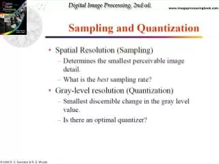
14. Sampling • sampling = the spacing of discrete values in the domain of a signal. • sampling-rate = how many samples are taken per unit of each dimension. e.g.,samples per second, frames per second

15. Quantization • Quantization = spacing of discrete values in the range of a signal. • Usually thought of as the number of bits per sample of the signal. e.g., 1, 8, 24 bit images, 16-bit audio.

16. Digital Image Representation • A digital image is an image f(x,y) that has been digitized both in spatial coordinates and brightness. • The value of f at any point (x,y) is proportional to the brightness (or gray level) of the image at that point.

17. 2D Image Sensor

18. Coordinate Conversion used in this book

19. Digital Image Representation

20. Digital Image Acquisition Process

21. Sampling and Quantization

22. Example of Digital Image

23. Sampling Effect

24. Sampling Effect

25. Chapter 2: Digital Image Fundamentals

26. Quantization Effect

27. Quantization Effect • if the gray scale is not enough, the smooth area will be affected. • False contouring can occur on the smooth area which has fine gray scales.

28. Light-intensity function • image refers to a 2D light-intensity function, f(x,y) • the amplitude of f at spatial coordinates (x,y) gives the intensity (brightness) of the image at that point. • light is a form of energy thus f(x,y) must be nonzero and finite. • 0 < f(x,y) < ∞

29. Illumination and Reflectance • The basic nature of f(x,y) may be characterized by 2 components: • the amount of source light incident on the scene being viewed Illumination, i(x,y) • the amount of light reflected by the objects in the scene  Reflectance, r(x,y)

30. Illumination and Reflectance f(x,y) = i(x,y)r(x,y) • i(x,y): • determined by the nature of the light source • bounded by 0 < i(x,y) < ∞ • r(x,y) : • determined by the nature of the objects • bounded by 0 < r(x,y) < 1

31. Gray Level • we call the intensity of a monochrome image f at coordinate (x,y) the gray level (l) of the image at that point. • thus, l lies in the range Lmin ≤ l ≤ Lmax • Lminand Lmaxare positive and finite. • gray scale = [Lmin, Lmax] • common practice, shift the interval to [0, L] • 0 = black , L = white

32. Resolution • Resolution (how much you can see the detail of the image) depends on sampling and gray levels. • the bigger the sampling rate (n) and the gray scale (g), the better the approximation of the digitized image from the original. But the size of the image gets bigger

33. Non-uniform Sampling • For a fixed value of spatial resolution, the appearance of the image can be improved by using adaptive sampling rates. • Fine sampling • Required in the neighborhood of sharp gray-level transitions. • Coarse sampling • Utilized in relatively smooth regions.

34. Chapter 2: Digital Image Fundamentals

35. Chapter 2: Digital Image Fundamentals For the images with a large amount of detail only a few gray levels may be needed.

36. Non-uniform Quantization • unequally spaced levels in quantization process influences on the decreasing the number of gray level. • use few gray levels in the neighborhood of boundaries. • use more gray levels on smooth area in order to avoid the “false contouring”.

37. Basic Relationship among pixels • Neighbors of a pixel • Connectivity • Labeling of Connected Components • Distance Measures • Arithmetic/Logic Operations

38. Neighbors of a Pixels

39. Connectivity • Let V be the set of gray-level values used to defined connectivity • 4-connectivity : • 2 pixels p and q with values from V are 4-connected if q is in the set N4(p) • 8-connectivity : • 2 pixels p and q with values from V are 8-connected if q is in the set N8(p) • m-connectivity (mixed connectivity): • 2 pixels p and q with values from V are m-connected if • q is in the set N4(p) or • q is in the set ND(p) and the set N4(p)∩N4(q) is empty. • (the set of pixels that are 4-neighbors of both p and q whose values are from V )

40. Example of Connectivity Path 8 neighbors m neighbors • m-connectivity eliminates the multiple path • connections that arise in 8-connectivity.

41. Path • a path from pixel p with coordinates (x,y) to pixel q with coordinates (s,t) is a sequence of distinct pixels with coordinates (x0,y0),(x1,y1),…(xn,yn) , where (x0,y0) = (x,y) , (xn,yn) = (s,t) and (xi,yi) is adjacent to (xi-1,yi-1) • n is the length of the path • we can define 4-,8-, or m-paths depending on type of adjacency specified.

42. Adjacent • A pixel p is adjacent to a pixel q if they are connected. • Two image area subsets S1 and S2 are adjacent if some pixel in S1 is adjacent to some pixel S2.

43. Labeling 1 • Scan the image from left to right • Let p denote the pixel at any step in the scanning process. • Let r denote the upper neighbor of p. • Let t denote the left-hand neighbors of p, respectively. • When we get to p, points r and t have already been encountered and labeled if they were 1’s. r t p

44. Labeling 2 • if the value of p = 0, move on. • if the value of p = 1, examine r and t. • if they are both 0, assign a new label to p. • if only one of them is 1, assign its label to p. • if they are both 1 • if they have the same label, assign that label to p. • if not, assign one of the labels to p and make a note that the two labels are equivalent. (r and t are connected through p). • At the end of the scan, all points with value 1 have been labeled. • Do a second scan, assign a new label for each equivalent labels.

45. Labeling with 8 connected components • do the same way but examine also the upper diagonal neighbors of p. • if p is 0, move on. • if p is 1 • if all four neighbors are 0, assign a new label to p. • if only one of the neighbors is 1, assign its label to p. • if two or more neighbors are 1, assign one of the label to p and make a note of equivalent classes. • after complete the scan, do the second round and introduce a unique label to each equivalent class.

46. Distance Measures • for pixel p, q and z with coordinates (x,y), (s,t) and (u,v) respectively, • D is a distance function or metric if • (a) D(p,q) ≥ 0 ; D(p,q) = 0 iff p=q • (b) D(p,q) = D(q,p) • (c) D(p,z) ≤ D(p,q) + D(q,z)

47. Euclidean Distance

48. City-Block Distance

49. Chessboard Distance

50. distances of m-connectivity of the path between 2 pixels depends on values of pixels along the path. e.g., if only connectivity of pixels valued 1 is allowed. find the m-distance between p and p4 p3 p4 0 1 1 1 1 1 p1 p2 0 1 0 1 1 1 p 1 1 1 d = 2 d=3 d=4 M-connectivity distances