Chapter 2 Digital Image Fundamentals

1. Chapter 2Digital Image Fundamentals 國立雲林科技大學 資訊工程研究所 張傳育(Chuan-Yu Chang ) 博士 Office: EB 212 TEL: 05-5342601 ext. 4337 E-mail: chuanyu@yuntech.edu.tw Website: MIPL.yuntech.edu.tw

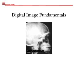
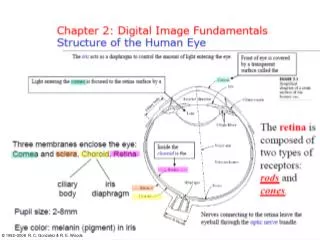
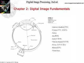
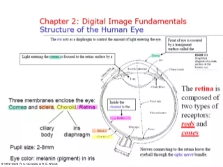
2. Structure of the Human Eye 角膜 虹膜 睫狀體 睫狀肌 水晶體 光受體有兩種： 1.錐狀體(cones) 600-700萬,對色彩很 靈敏，白晝視覺。 2.桿狀體(rods) 7500-1500萬,對低亮度 很靈敏，夜視視覺。 玻璃體 視網膜 盲點 中央凹 鞏膜 脈絡膜

3. Structure of the Human Eye (cont.) • Distribution of rods and cones in the retina

4. Image Formation in the Eye • Graphical representation of the eye looking at a palm tree

5. Image Formation in the Eye (cont.) • Brightness adaptation and Discrimination

6. Image Formation in the Eye (cont.)

7. Image Formation in the Eye (cont.) • Typical Weber ratio as a function of intensity

8. Image Formation in the Eye (cont.)

9. Image Formation in the Eye (cont.)

10. Image Formation in the Eye (cont.) Optical illusion

11. Light and the Electromagnetic Spectrum

12. Light and the Electromagnetic Spectrum (cont.) =c/v : wavelength v: frequency c: speed of light (2.998*108 m/s)

13. Chapter 2: Digital Image Fundamentals

14. Chapter 2: Digital Image Fundamentals

15. Chapter 2: Digital Image Fundamentals

16. Chapter 2: Digital Image Fundamentals Digital Image Acquisition Process

17. Chapter 2: Digital Image Fundamentals • Image Sampling and Quantization • To create a digital image, we need to convert the continuous sensed data into digital form. This involves two processes: • Sampling • Digitizing the coordinate values • Quantization • Digitizing the amplitude values

18. Chapter 2: Digital Image Fundamentals Image Sampling and Quantization

19. Chapter 2: Digital Image Fundamentals

20. Chapter 2: Digital Image Fundamentals • Representing Digital Images • The result of sampling and quantization is a matrix of real numbers.

21. Chapter 2: Digital Image Fundamentals

22. Chapter 2: Digital Image Fundamentals • Spatial Resolution • The smallest discernible detail in an image. • Line pair • Size: 1024*1024

23. Chapter 2: Digital Image Fundamentals

24. Chapter 2: Digital Image Fundamentals • Gray-Level Resolution • The smallest discernible change in gray level. • The # of gray levels is usually an integer power of 2.

25. Chapter 2: Digital Image Fundamentals False contouring

26. Chapter 2: Digital Image Fundamentals • Isopreference curves (Huang, 1965) • Quantify experimentally the effects on image quality produced by varying N and k simultaneously. • Points lying on an isopreference curves correspond to images of equal subjective quality • Isopreference curves tend to become more vertical as the detail in the image increase. • For image with a large amount of detail only a few gray levels may be needed.

27. Chapter 2: Digital Image Fundamentals • Aliasing and Moire Patterns • Functions whose area under the curve is finite can be represented in terms of sine and cosines of various frequencies. • Suppose that this highest frequency is finite and that the function is of unlimited duration. • The Shannon sampling theorem tells us, if the function is sampled at a rate equal to or greater than twice its highest frequency, it is possible to recover completely the original function from its samples. • If the function is undersampled, then a phenomenon called aliasing corrupted the sampled image.

28. Chapter 2: Digital Image Fundamentals • In practice, it is impossible to satisfy the sampling theorem. • We can only work with sampled data that are finite in duration. • Multiplying the unlimited function by a “gating function” that is valued 1 for some interval and 0 elsewhere. • The gating function itself has frequency components that extend to infinity. • The principal approach for reducing the aliasing effects on an image is to reduce its high-frequency components by blurring the image prior to sampling.

29. Chapter 2: Digital Image Fundamentals • Zooming • Zooming may be views as oversampling. • Zooming requires two steps: • Step 1: the creation of new pixel location. • Step 2: the assignment of gray level to those new locations. • Nearest neighbor interpolation • Look for the closest pixel in the original image and assign its gray level to the new pixel in the grid. • Pixel replication • To double the size of an image, we can duplicate each column/ row • Biliner interpolation • Using the four nearest neighbors of a point.

30. Zooming (cont.) • Example 2.4 • Using nearest neighbor gray-level/ bilinearinterpolation

31. Chapter 2: Digital Image Fundamentals • Shrinking • Shrinking may be views as undersampling. • Row-column deletion • To shrink an image by one-half, we delete every other row and column.

32. p p p Some basic relationships between pixels • Some basic relationships between pixels • Neighbors of a pixel • 4-neighbors of p: N4(p) • (x+1, y), (x-1, y), (x, y+1), (x, y-1) • diagonal-neighbors of p: ND(p) • (x+1, y+1), (x+1, y-1), (x-1, y+1), (x-1, y-1) • 8-neighbors of p: N8(p) • (x+1, y), (x-1, y), (x, y+1), (x, y-1), (x+1, y+1), (x+1, y-1), (x-1, y+1), (x-1, y-1)

33. Some basic relationships between pixels (cont.) • If two pixels are connected, it must be determined • If they are neighbors and • If their gray levels satisfy a specified criterion of similarity.

34. Some basic relationships between pixels (cont.) • Adjacency: two pixels p and q with value from V are • 4-adjacency: if q is in the set N4(p). • 8-adjacency : if q is in the set N8(p). • m-adjacency: if (i) q is in N4(p)or (ii) q is in ND(p)and the set N4(p)∩N4(q)has no pixels whose values are from V. • To eliminate the ambiguities arise when 8-adjacency is used.

35. Some basic relationships between pixels (cont.) • Digital path (or curve) • Path is a sequence of distinct pixels with coordinates • (x0, y0), (x1, y1),…,(xn, yn) • n is the length of the path • If (x0, y0)=(xn, yn), the path is closed path. • Connectivity • Connected component • Regions • If R is a connected set. • Boundary (border, contour) • The boundary of a region R is the set of pixels in the region that have one or more neighbors that are not in R. • The boundary of a finite region forms a closed path • Edge • The edges are formed from pixels with derivative values that exceed a preset threshold.

36. 2 1 0 1 2 2 1 2 2 1 2 2 2 Some basic relationships between pixels (cont.) • Distance measure • Pixels:p=(x,y), q=(s,t), z=(v, w) • Euclidean distance between p and qis defined as • D4 distance (city-block distance) between p and qis defined as

37. Some basic relationships between pixels (cont.) • D8 distance (chessboard distance) between p and q is defined as • Example: D8 distance<=2 2 2 2 2 2 2 1 1 1 2 2 1 0 1 22 1 1 1 22 2 2 2 2

38. Some basic relationships between pixels (cont.) • Dm distance between p and q is defined as the shortest m-path between the points. • Assume that p, p2, and p4 are 1. p3 p4p1 p2p 1p40p2p m-path=3 0p40p2p 1p41p2p m-path=4 m-path=2 0p41p2p m-path=3