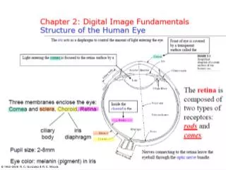
Chapter 2: Digital Image Fundamentals
740 likes | 1.01k Vues
Chapter 2: Digital Image Fundamentals. HVS cannot operate over 10 ^ 10 orders of magnitude dynamic range simultaneously Total range of distinct intensity levels eye can discriminate simultaneously is small

Chapter 2: Digital Image Fundamentals
E N D
Presentation Transcript
HVS cannot operate over 10 ^ 10 orders of magnitude dynamic range simultaneously • Total range of distinct intensity levels eye can discriminate simultaneously is small • For given conditions, the current visual sensitivity of HVS is called “brightness adaptation”.
incremental illumination Δ I appears in the form of a short duration flash
Light and EM Spectrum • The colors that humans perceive in an object are determined by the nature of the light reflected from the object. e.g. green objects reflect light with wavelengths primarily in the 500 to 570 nm range while absorbing most of the energy at other wavelength
Monochromatic light: void of color Intensity is the only attribute, from black to white Monochromatic images are referred to as gray-scale images • Chromatic light bands: 0.43 to 0.79 um The quality of a chromatic light source: Radiance: total amount of energy Luminance (lm): the amount of energy an observer perceives from a light source Brightness: a subjective descriptor of light perception that is impossible to measure. It embodies the achromatic notion of intensity and one of the key factors in describing color sensation.
Illumination Lumen —A unit of light flow or luminous flux Lumen per square meter (lm/m2) —The metric unit of measure for illuminance of a surface On a clear day, the sun may produce in excess of 90,000 lm/m2 of illumination on the surface of the Earth On a cloudy day, the sun may produce less than 10,000 lm/m2 of illumination on the surface of the Earth On a clear evening, the moon yields about 0.1 lm/m2 of illumination The typical illumination level in a commercial office is about 1000 lm/m2 Some Typical Ranges of illumination
Reflectance 0.01 for black velvet 0.65 for stainless steel 0.80 for flat-white wall paint 0.90 for silver-plated metal 0.93 for snow Some Typical Ranges of Reflectance
Discrete intensity interval [0, L-1], L=2k • The number b of bits required to store a M × N digitized image b = M × N × k
Spatial resolution — A measure of the smallest discernible detail in an image — stated with line pairs per unit distance, dots (pixels) per unit distance, dots per inch (dpi) Intensity resolution — The smallest discernible change in intensity level — stated with 8 bits, 12 bits, 16 bits, etc. Spatial and Intensity Resolution
Interpolation — Process of using known data to estimate unknown values e.g., zooming, shrinking, rotating, and geometric correction Interpolation(sometimes calledresampling)—an imaging method to increase (or decrease) the number of pixels in a digital image. Some digital cameras use interpolation to produce a larger image than the sensor captured or to create digital zoom http://www.dpreview.com/learn/?/key=interpolation Image Interpolation
Image Interpolation: Nearest Neighbor Interpolation f1(x2,y2) = f(round(x2), round(y2)) =f(x1,y1) f(x1,y1) f1(x3,y3) = f(round(x3), round(y3)) =f(x1,y1)
The intensity value assigned to point (x,y) is obtained by the following equation The sixteen coefficients are determined by using the sixteen nearest neighbors. http://en.wikipedia.org/wiki/Bicubic_interpolation Image Interpolation: Bicubic Interpolation
Noiseless image: f(x,y) Noise: n(x,y) (at every pair of coordinates (x,y), the noise is uncorrelated and has zero average value) Corrupted image: g(x,y) g(x,y) = f(x,y) + n(x,y) Reducing the noise by adding a set of noisy images, {gi(x,y)} Example: Addition of Noisy Images for Noise Reduction
Example: Addition of Noisy Images for Noise Reduction • In astronomy, imaging under very low light levels frequently causes sensor noise to render single images virtually useless for analysis. • In astronomical observations, similar sensors for noise reduction by observing the same scene over long periods of time. Image averaging is then used to reduce the noise.
Black regions in (c) shows no difference Non black is regions where they are different
Mask h(x,y): an X-ray image of a region of a patient’s body Live images f(x,y): X-ray images captured at TV rates after injection of the contrast medium Enhanced detail g(x,y) g(x,y) = f(x,y) - h(x,y) The procedure gives a movie showing how the contrast medium propagates through the various arteries in the area being observed. An Example of Image Subtraction: Mask Mode Radiography