Remote Sensing of Snow
570 likes | 1.2k Vues
Remote Sensing of Snow. Presented to: ENSC 454/654 Presented by: Jinjun Tong Date: January 22, 2009. Outline. Fundamentals of remote sensing Satellites and sensors Application of remote sensing Remotely sensed snow distribution in the Quesnel River Basin (QRB).

Remote Sensing of Snow
E N D
Presentation Transcript
Remote Sensing of Snow Presented to: ENSC 454/654 Presented by: Jinjun Tong Date: January 22, 2009
Outline • Fundamentals of remote sensing • Satellites and sensors • Application of remote sensing • Remotely sensed snow distribution in the Quesnel River Basin (QRB)
Definition of Remote Sensing Several of the human senses gather their awareness of the external world almost entirely by perceiving a variety of signals, either emitted or reflected, actively or passively, from objects that transmit this information in waves or pulses.
Remote Sensing is a technology for sampling electromagnetic radiation to acquire and interpret non-immediate geospatial data from which to extract information about features, objects, and classes on the Earth's land surface, oceans, and atmosphere (and, where applicable, on the exteriors of other bodies in the solar system, or, in the broadest framework, celestial bodies such as stars and galaxies).
Energy Source or Illumination (A) • Radiation and the Atmosphere (B) • Interaction with the Target (C) • Recording of Energy by the Sensor (D) • Transmission, Reception, and Processing (E) • Interpretation and Analysis (F) • Application (G)
ultraviolet Visible
Infrared Microwaves
Interactions with the Atmosphere Scattering Absorbing
Those areas of the spectrum which are not severely influenced by atmospheric absorption and thus, are useful to remote sensors, are calledatmospheric windows
Target Interactions • Absorption (A) occurs when radiation (energy) is absorbed into the target while transmission (T) occurs when radiation passes through a target. Reflection (R) occurs when radiation "bounces" off the target and is redirected.
water and vegetation may reflect somewhat similarly in the visible wavelengths but are almost always separable in the infrared.
Passive vs. Active Remote Sensing Passive Sensing Active Sensing
Satellites and Sensors • In order for a sensor to collect and record energy reflected or emitted from a target or surface, it must reside on a stable platform removed from the target or surface being observed. Platforms for remote sensors may be situated on the ground, on an aircraft or balloon (or some other platform within the Earth's atmosphere), or on a spacecraft or satellite outside of the Earth's atmosphere. Although ground-based and aircraft platforms may be used, satellites provide a great deal of the remote sensing imagery commonly used today.
Satellite Orbits Geostationary orbits Sun-synchronous orbits Near-polar orbits
Weather Satellites/Sensors • TIROS-1(launched in 1960 by the United States) • GOES (Geostationary Operational Environmental Satellite) -GOES-1 (launched 1975), GOES-8 (launched 1994) • Advanced Very High Resolution Radiometer(NOAA AVHRR)(sun-synchronous, near-polar orbits) • FengYun-1, FengYun-2, FengYun-3, FengYun-4 (China) • GMS (Japan) • Meteosat (European)
Land Observation Satellites/Sensors • Landsat (Landsat-1 was launched by NASA in 1972, near-polar, sun-synchronous orbits). -Return Beam Vidicon (RBV), MultiSpectral Scanner (MSS), Thematic Mapper (TM) • SPOT(SPOT-1 was launched by France in 1986, sun-synchronous, near-polar orbits) -Twin high resolution visible (HRV) • Multispectral Electro-optical Imaging Scanner(MEIS II) Compact Airborne Spectrographic Imager(CASI)(airborne sensors)(Canada) • CBERS-1 (China & Brazil)
Marine Observation Satellites/Sensors • Nimbus-7 satellite (launched by NOAA in 1978) -Coastal Zone Colour Scanner (CZCS) • Marine Observation Satellite (MOS-1)( launched by Japan in February, 1987) -a four-channel Multispectral Electronic Self-Scanning Radiometer (MESSR), -a four-channel Visible and Thermal Infrared Radiometer (VTIR), -a two-channel Microwave Scanning Radiometer (MSR) • SeaWiFS (Sea-viewing Wide-Field-of View Sensor), SeaStar spacecraft, (NASA) • HY-1 (launched by China in 2001)
Data Reception, Transmission, and Processing In Canada, CCRS operates two ground receiving stations - one at Cantley, Québec (GSS), just outside of Ottawa, and another one at Prince Albert, Saskatchewan (PASS)
Applications of Remote Sensing • Agriculture • Forestry • Geology • Oceans & Coastal Monitoring • Mapping • Hydrology • Land Cover & Land Use • Snow Ice
Agriculture • crop type classification • crop condition assessment • crop yield estimation • mapping of soil characteristics • mapping of soil management practices • compliance monitoring (farming practices)
Forestry • reconnaissance mapping: -forest cover type discrimination -agroforestry mapping • Commercial forestry: -clear cut mapping / regeneration assessment -burn delineation -infrastructure mapping / operations support -forest inventory -biomass estimation -species inventory • Environmental monitoring: -deforestation (rainforest, mangrove colonies) -species inventory -watershed protection (riparian strips) -coastal protection (mangrove forests) -forest health and vigour
Geology • surficial deposit / bedrock mapping • lithological mapping • structural mapping • sand and gravel (aggregate) exploration/ xploitation • mineral exploration • hydrocarbon exploration • environmental geology • geobotany • baseline infrastructure • sedimentation mapping and monitoring • event mapping and monitoring • geo-hazard mapping • planetary mapping
Oceans & Coastal Monitoring • Ocean pattern identification • Storm forecasting • Fish stock and marine mammal assessment • Oil spill • Shipping • Intertidal zone
Mapping • planimetry • digital elevation models (DEM's) • baseline thematic mapping/topographic mapping
Hydrology • wetlands mapping and monitoring, • soil moisture estimation, • snow pack monitoring / delineation of extent, • measuring snow depth, • determining snow-water equivalent, • river and lake ice monitoring, • flood mapping and monitoring, • glacier dynamics monitoring (surges, ablation) • river /delta change detection • drainage basin mapping and watershed modelling • irrigation canal leakage detection • irrigation scheduling
Land Cover & Land Use • natural resource management • wildlife habitat protection • baseline mapping for GIS input • urban expansion / encroachment • routing and logistics planning for seismic / • exploration / resource extraction activities • damage delineation (tornadoes, flooding, • volcanic, seismic, fire) • legal boundaries for tax and property evaluation • target detection - identification of landing strips, • roads, clearings, bridges, land/water interface
Sea Ice • ice concentration • ice type / age /motion • iceberg detection and tracking • surface topography • tactical identification of leads: navigation: safe shipping routes/rescue • ice condition (state of decay) • historical ice and iceberg conditions and dynamics for planning purposes • wildlife habitat • pollution monitoring • meteorological / global change research
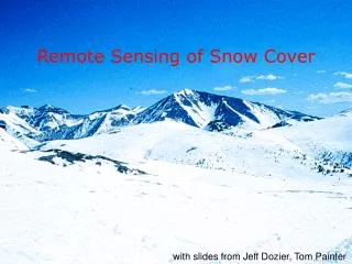
Remotely sensed snow distribution and its relationships with the hydrometeorology in the QRB, Canada
Outline • Research background and area • Data processing methods • Evaluation of Moderate Resolution Imaging Spectroradiometer (MODIS) data • Snow distribution in the QRB • Relationships between snow cover extent (SCE), snow cover fraction (SCF), snow cover duration (SCD), topography, streamflow, and climate change. • Conclusions
DEM in the QRB • Snow plays a vital role in the energy and water budgets of drainage basins. • the SCE and snow water equivalent (SWE) are important parameters for various hydrologic models. • The QRB is one of 13 main sub-watersheds in Fraser River Basin, which is one of the world's most productive salmon river systems with five salmon species and 65 other species of fish.
Data • MODIS daily and 8-day SCE • Global land one-kilometer base elevation (GLOBE) DEM • Daily streamflow of Quesnel River • Daily snow depth, temperature and precipitation of nine ground stations
EOS-MODIS Let’s watch the video about the EOS-MODIS instruments first
Snowmap • The snow-mapping algorithm (Snowmap) employs a Normalized Difference Snow Index (NDSI) to identify and classify snow on a pixel-by-pixel basis. Reflectance of snow and ice
NDSI • A Normalized Difference Snow Index (NDSI) is computed from Band 4 (green) and Band 6 (SWIR): • Snow is determined if: NDSI ≥ 0.4, and the reflectance in Band 2 (near-IR) ≥ 0.11, and Band 4 (green) ≥ 0.10, to eliminate water and other dark surfaces from being classified as snow. A Normalized Difference Vegetation Index (NDVI) is computed from MODIS Band 1 (Red) and Band 2, and the NDSI and NDVI are used together to map snow in dense forests.
The NDSI is also used for MODIS sea ice products. In regions illuminated by the sun, the NDSI is used to differentiate sea ice from open water. A second method, one based on Ice Surface Temperature (IST), is also used for detection of sea ice. This is especially useful in areas lacking solar illumination. MODIS Bands 31 and 32, near 11.6 μm, are used in a split-window technique to derive IST, utilizing coefficients specific to sea ice. • Let’s watch the animation shows the global advance and retreat of daily snow cover along with daily sea ice surfacetemperature over the Northern Hemisphere from September 2002 through May 2003.
Reclassify images as snow, no snow, and cloud Central point P Cloud P=Original value No Yes Cloud for all other 8 points P=Cloud Yes No Snow>=No snow No P=No snow Yes P=Snow Data Processing Spatial filter method points Flow chart of spatial filter method
Comparison of snow maps of MOD10A1, MOD10A2, and SF in the QRB within the same period and 8-day annual average cloud coverage of MOD10A1, MOD10A2, and SF from 2000-2007 in the QRB.
Evaluation of MODIS data MODIS Ground Accuracy of different MODIS snow data
Relationships between topography, SCF and SCD Annual cycle of the SCF distribution in different elevation bands, 2000-2007. The SCD for different periods across the QRB based on the MOD10A2 (left) and SF (right) products, 2001-2007. The SCD days for the entire year equal 3 times the values in the legend.
The mean (left) and standard deviations (right) of SCDs for 10-m elevation bands for 3 seasons based on the MOD10A2 and SF products, 2001-2007. The correlation coefficients between SCDs and elevations within different periods (p<0.001) and the corresponding d(SCD)/dz (days (100 m)-1) in parentheses.
(a) The mean elevational dependence of snow cover fraction (SCF) for the months of February to July, 2000-2007. (b) The mean (points) and standard deviation (bars) of the rate of change in SCF at different elevations, 26 February to 26 June, 2000-2007. The average annual cycle of snow cover fraction distribution in different slope and aspect bands, 2000-2007.
Relationships between runoff, SCF and SCE Lagged correlation coefficients between 8-day maximum SCE in the QRB and streamflow of QR during snow melt seasons from 2000-2007. The 8-day MODIS maximum snow cover fraction of the QRB and the corresponding 8-day runoff at Quesnel gauge station from February 26,2000 to December 31,2007.
Scatter plots between (normalized) SCE and (normalized) streamflow during snow ablation seasons from 2000-2007 in the QRB
MOD10A2 Relationships between SCF, runoff and climate change Correlation coefficients (a) and scatter plot (b) between average temperature within different periods and SCF50% and scatter plot (c) between SCF50% and R50% during snow melt seasons from 2000-2007 in the QRB.
Conclusions • Spatial filter method can decrease the cloud cover fraction from average 15% to 10% with increasing the accuracy of the MODIS snow products. • Spatial filter method can improve the analyses between the MODIS snow products and other characteristics such as streamflow, SCE, SCF and SCD. • There are significant correlations between the SCE and streamflow of QRB during the snow melt seasons with a correlation coefficient -0.8 (p<0.001).
The snow melt process is highly correlated with the mean temperature in the QRB with a correlation coefficient -0.85 (p<0.01). The runoff has significant linear relationship with SCF with a correlation coefficient 0.82 (p<0.01). • The SCD is correlated with the elevations significantly in QRB with correlation coefficient over -0.95 (p<0.001). There is perennial snow over 2500 m in the QRB.