Methodologies for Performance Simulation of Super-scalar Out-of-Order Processors
310 likes | 440 Vues
This document surveys advanced methodologies for performance simulation of super-scalar Out-of-Order (OOO) processors. It emphasizes both functional and performance simulators, focusing on design space exploration and evaluation of existing or proposed hardware. Key methodologies include Hybrid Statistical and Symbolic Simulation (HLS) and Basic Block Distribution Analysis (BBDA). These techniques aim to improve simulation efficiency while addressing challenges like long simulation times and vast design spaces. The findings highlight the potential of combining various simulation approaches to achieve accurate performance predictions.

Methodologies for Performance Simulation of Super-scalar Out-of-Order Processors
E N D
Presentation Transcript
Methodologies for Performance Simulation of Super-scalar OOO processors Srinivas Neginhal Anantharaman Kalyanaraman CprE 585: Survey Project
Architectural Simulators • Explore Design Space • Evaluate existing hardware, or Predict performance of proposed hardware • Designer has control Functional Simulators: Model architecture (programmers’ focus) Eg., sim-fast, sim-safe Performance Simulators: Model microarchitecture (designer’s focus) Eg., cycle-by-cycle (sim-outoforder)
Simulation Issues • Real-applications take too long for a cycle-by-cycle simulation • Vast design space: • Design Parameters: • code properties, value prediction, dynamic instruction distance, basic block size, instruction fetch mechanisms, etc. • Architectural metrics: • IPC/ILP, cache miss rate, branch prediction accuracy, etc. • Find design flaws + Provide design improvements • Need a “robust” simulation methodology !!
Two Methodologies • HLS • Hybrid: Statistical + Symbolic • REF: • HLS: Combining Statistical and Symbolic Simulation to Guide Microprocessor Designs. M. Oskin, F. T. Chong and M. Farrens. Proc. ISCA. 71-82. 2000. • BBDA • Basic block distribution analysis • REF: • Basic Block Distribution Analysis to Find Periodic Behavior and Simulation Points in Applications. T. Sherwood, E. Perelman and B. Calder. Proc. PACT. 2001.
HLS: An Overview • A hybrid processor simulator Statistical Model HLS Performance Contours spanned by design space parameters Symbolic Execution What can be achieved? Explore design changes in architectures and compilers that would be impractical to simulate using conventional simulators
HLS: Main Idea Synthetically generated code Application code Statistical Profiling Instruction stream, data stream Structural Simulation of FU, issue pipeline units • Code characteristics: • basic block size • Dynamic instruction distance • Instruction mix • Architecture metrics: • Cache behavior • Branch prediction accuracy
Statistical Code Generation • Each “synthetic instruction” contains the following parameters based on the statistical profile: • Functional unit requirements • Dynamic instruction distances • Cache behavior
Validation of HLS against SimpleScalar • For varying combinations of design parameters: • Run original benchmark code on SimpleScalar (use sim-outoforder) • Run statistically generated code on HLS • Compare SimpleScalar IPC vs. HLS IPC
Validation: Single- and Multi-value correlations IPC vs. L1-cache hit rate For SPECint95: HLS Errors are within 5-7% of the cycle-by-cycle results !!
HLS: Code PropertiesBasic Block Size vs. L1-Cache Hit Rate • Correlation suggests that: • Increasing block size helps only when L1 cache hit rate is >96% or <82%
HLS: Value Prediction GOAL: Break True Dependency Stall Penalty for mispredict vs. Value Prediction Knowledge DID vs. Value predictability
HLS: Conclusions • Low error rate only on SPECint95 benchmark suite. High error rates on SPECfp95 and STREAM benchmarks • Findings: by R. H. Bell et. Al, 2004 • Reason: • Instruction-level granularity for workload • Recommended Improvement: • Basic block-level granularity
Basic Block Distribution Analysis Basic Block Distribution Analysis to Find Periodic Behavior and Simulation Points in Applications. T. Sherwood, E. Perelman and B. Calder. Proc. PACT. 2001.
Introduction • Goal • To capture large scale program behavior in significantly reduced simulation time. • Approach • Find a representative subset of the full program. • Find an ideal place to simulate given a specific number of instructions one has to simulate • Accurate confidence estimation of the simulation point. Simulation Points Period Program Execution
Program Behavior • Program behavior has ramifications on architectural techniques. • Program behavior is different in different parts of execution. • Initialization • Cyclic behavior (Periodic) • Cyclic Behavior is not representative of all programs. • Common case for compute bound applications.
BBDA Basics • Fast profiling is used to determine the number of times a basic block executes. • Behavior of the program is directly related to the code that it is executing. • Profiling gives a basic block fingerprint for that particular interval of time. • The interval chosen is ideally a representative of the full execution of the program. • Profiling information is collected in intervals of 100 million instructions.
Basic Block Vector BBV for Interval i: B1 B2 Frequency Interval i … • BBV = Fingerprint of an interval • Varying size intervals • A BBV collected over an interval of N times 100 million instructions is a BBV of duration N. Bx
Target BBV • BBVs are normalized • Each element divided by the sum of all elements. • Target BBV • BBV for the entire execution of the program. • Objective • Find a BBV of smallest duration “similar” to Target BBV.
Basic Block Vector Difference • Difference between BBVs • Euclidean Distance • Manhattan Distance
Basic Block Difference Graph • Plot of how well each individual interval in the program compares to the target BBV. • For each interval of 100 million instructions, we create a BBV and calculate its difference from target BBV. • Used to • Find the end of initialization phase. • Find the period for the program.
Initialization • Initialization is not trivial. • Important to simulate representative sections of the initialization code. • Detection of the end of the initialization phase is important. • Initialization Difference Graph • Initial Representative Signal - First quarter of BB Difference graph. • Slide it across BB difference graph. • Difference calculated at each point for first half of BBDG. • When IRS reaches the end of the initialization stage on the BB difference graph, the difference is maximized.
Period • Period Difference Graph • Period Representative Signal • Part of BBDG, starting from the end of initialization to ¼th the length of program execution. • Slide across half the BBDG. • Distance between the minimum Y-axis points is the period. • Using larger durations of a BBV creates a BBDG that emphasizes larger periods.
Summary of Results • IPC of chosen period vs. IPC of the full execution Differed by 5% • BBV based technique (to be continued…)
Characterizing Program Behavior Through Clustering Automatically characterizing Large Scale Program Behavior. T. Sherwood, E. Perelman, G. Hamerly and B. Calder. ASPLOS 2002
Clustering Approach #1 P1 #2 P2 Clustering N BBVs Multiple Simulation Points … … #K Pk Clusters
Clustering (k-means) • Goal is to divide a set of points into groups such that points within each group are similar to one another by a desired metric. • Input: N points in D-dimensional space • Output: A partition of k clusters • Algorithm: • Randomly choose k points as centroids (initialization) • Compute cluster membership of each point based on its distance from each centroid • Compute new centroid for each cluster • Iterate steps 2 and 3 until convergence Runtime complexity affected by the “curse of dimensionality”
Random Projection • Reduce the dimension of the BBVs to 15 • Dimension Selection • Dimension Reduction • Random Linear Projection.
BBDA: Conclusions • BBDA provides better sensitivity and lower performance variation in phases • Other related work such as instruction working set technique provides higher “stability”