Download

1 / 48
480 likes | 521 Vues
The Capital Budgeting Decision. 12. Chapter Outline. Capital budgeting decision. Cash flows and capital budgeting. Methods for ranking investments Payback methods Internal rate of return Net present value. Discount or cutoff rate.

E N D
Chapter Outline • Capital budgeting decision. • Cash flows and capital budgeting. • Methods for ranking investments • Payback methods • Internal rate of return • Net present value. • Discount or cutoff rate. • After-tax operating benefits and tax shield benefits of depreciation.
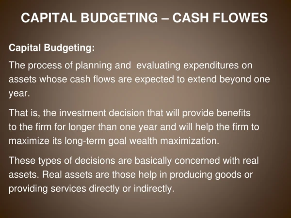
Capital Budgeting Decision • Involves planning of expenditures for a project with a minimum period of a year or longer. • Capital expenditure decisions requires: • Extensive planning and coordination of different departments. • Uncertainties are common in areas such as: • Annual costs and inflows, product life, economic conditions, and technological changes.
Administrative Considerations • Steps in the decision-making process: • Search for and discovery for investment opportunities. • Collection of data. • Evaluation and decision making. • Reevaluation and adjustment.
Accounting Flows versus Cash Flows • Capital budgeting decisions - emphasis remains on cash flow. • Depreciation (non cash expenditure) is added back to profit to determine the amount of cash flow generated. • An example shown in the next slide. • The emphasis is on the use of proper evaluation techniques for to make best economic choices and assure long term wealth.
Methods of Ranking Investment Proposals • Three methods used: • Payback method – although not sound conceptually, is often used. • Internal rate of return - more acceptable and commonly used. • Net present value - more acceptable and commonly used.
Payback Method • Time required to recoup the initial investment. • Table 12-3, using Investment A: • There is no consideration of inflows after the cutoff period. • The method fails to consider the concept of the time value of money. Year Early Returns Late Returns 1……….. $9,000 $1,000 2……….. $1,000 $9,000 3……….. $1,000 $1,000
Payback Method (cont’d) • Advantages: • Easy to understand and emphasizes liquidity. • Must recoup the initial investment quickly or it will not qualify. • Rapid payback preferred in industries characterized by dynamic technological environment. • Shortcomings: • Fails to discern the optimum or most economic solution to a capital budgeting problem.
Internal Rate of Return • Requires the determination of the yield on an investment with subsequent cash inflows. • Assuming that a $1,000 investment returns an annuity of $244 per annum for five years, provides an internal rate of return of 7%: • Dividing the investment (present value) by the annuity: (Investment) = $1,000 = 4.1 (PVIFA) (Annuity) $244 • The present value of an annuity (given in Appendix D) shows that the factor of 4.1 for five years indicates a yield of 7%.
Determining Internal Rate of Return Cash Inflows (of $10,000 investment) Year Investment A Investment B 1……………… $5,000 $1,500 2……………… $5,000 $2,000 3……………… $2,000 $2,500 4……………… $5,000 5……………… $5,000 • To find a beginning value to start the first trial, the inflows are averaged out as though annuity was really being received. $5,000 $5,000 $2,000 $12,000 ÷ 3 = $4,000
Determining Internal Rate of Return (cont’d) • Dividing the investment by the ‘assumed’ annuity value in the previous step, we have; (Investment) = $10,000 = 2.5 (PVIFA) (Annuity) $4,000 • The first approximation (derived from Appendix D) of the internal rate of return using; the factor falls between 9 and 10 percent; PVIFA factor = 2.5 n (period) = 3 • Averaging understates the actual IRR and the same method would overstate the IRR for Investment B. • Cash flows in the early years are worth more and increase the return, it is possible to gauge whether the first approximation is over- or under- stated.
Determining Internal Rate of Return (cont’d) • Using the trial and error approach, we use both 10% and 12% to arrive at the answer: Year 10% 1…….$5,000 X 0.909 = $4,545 2…….$5,000 X 0.826 = $4,130 3…….$2,000 X 0.751 = $1,502 $10,177 • (At 10%, the present value of the inflows exceeds $10,000 – we therefore use a higher discount rate). Year 12% 1…….$5,000 X 0.893 = $4,465 2…….$5,000 X 0.797 = $3,985 3…….$2,000 X 0.712 = $1,424 $9,874 • (At 12%, the present value of the inflows is less than $10,000 – thus the discount rate is too high).
Interpolation of the Results • The internal rate of return is determined when the present value of the inflows (PVI) equals the present value of the outflows (PVO). • The total difference in present values between 10% and 12% is $303. $10,177…… PVI @ 10% $10,177…….PVI @ 10% - $9,874…....PVI @ 12% - $10,000……(cost) $303 $177 • The solution is ($177/$303) percent of the way between 10 and 12 percent. Due to a 2% difference, the fraction is multiplied by 2% and the answer is added to 10% of the final answer of: 10% + ($177/$303) (2%) = 11.17% IRR. • The exact opposite of this conclusion is yielded for Investment B (14.33%).
Interpolation of the Results (cont’d) • The use of the internal rate of return requires the calculated selection of Investment B in preference to Investment A, the conclusion being exactly the opposite under the payback method. • The final selection of any project will also depend on the yield exceeding some minimum cost standard, such as the cost of capital to the firm. Investment A Investment B Selection Payback method……..2 years 3.8 years Quicker payback: Investment A Internal Rate of Return………11.17% 14.33% Higher yield: Investment B
Net Present Value • Discounting back the inflows over the life of the investment to determine whether they equal or exceed the required investment. • Basic discount rate is usually the cost of the capital to the firm. • Inflows must provide a return that at least equals the cost of financing those returns.
Net Present Value (cont’d) $10,000 Investment, 10% Discount Rate Year Investment A Year Investment B 1……… $5,000 X 0.909 = $4,545 1………. $1,500 X 0.909 = $1,364 2……… $5,000 X 0.826 = $4,130 2………. $2,000 X 0.826 = $1,652 3……… $2,000 X 0.751 = $1,502 3………. $2,500 X 0.751 = $1,878 $10,177 4………. $5,000 X 0,683 = $3,415 5………. $5,000 X 0.621 = $3,105 $11,414 Present value of inflows…..$10,177 Present value of inflows…..$11,414 Present value of outflows -$10,000 Present value of outflows -$10,000 Net present value……………..$177 Net present value…………...$1,414
Selection Strategy • For a project to be potentially accepted: • Profitability must equal or exceed the cost of capital. • Projects that are mutually exclusive: • Selection of one alternative will preclude selection of any other alternative. • Projects that are not mutually exclusive: • Alternatives that provide a return in excess of cost of capital will be selected.
Selection Strategy (cont’d) • In the case of the prior Investment A and B, assuming a capital of 10%, Investment B would be accepted if the alternatives were mutually exclusive, while both would clearly qualify if they were not so.
Selection Strategy (cont’d) • Assumption used: • Internal rate of return and net present value methods call for the same decision. • Exceptions to this generally common scenario are: • Both methods will accept or reject the same investments. • The two methods may give different answers in selecting the best investment from a range of acceptable alternatives.
Reinvestment Assumption • All inflows can be reinvested at the yield from a given investment. • Investments with very high IRR • May be unrealistic to assume that reinvestment can occur at a equally high rate. • Under the net present value method: • Allows for certain consistency.
The Reinvestment Assumption – Net Present Value ($10,000 Investment)
Modified Internal Rate of Return (MIRR) • Combines reinvestment assumption of the net present value method with the internal rate of return.
Modified Internal Rate of Return (MIRR) (cont’d) • Assuming $10,000 produces the following inflows for the next three years; • The cost of capital is 10%. • Determining the terminal value of the inflows at a growth rate equal to the cost of capital: • To determine the MIRR: PVIF = PV = $10,000 = .641 (Appendix B) FV $16,610
Capital Rationing • Artificial restraint set on the usage of funds that can be reinvested in a given period. • May be adopted because of: • Fearful of too much growth. • Hesitation to use external sources of funding. • Hinders a firm from achieving maximum profitability.
Net Present Value Profile • Allows the graphical representation of the net present value of a project at different discount rates. • To apply the net present value profile, three characteristics need to be looked into: • The net present value at a zero discount rate. • The net present value as determined by a normal discount rate (such as cost of capital). • The internal rate of return for the investments.
The Rules of Depreciation • Assets are classified according to nine categories. • Determine the allowable rate of depreciation write-off. • Modified accelerated cost recovery system (MACRS) represent the categories. • Asset depreciation range (ADR) is the expected physical life of the asset or class of assets.
The Tax Rate • Corporate tax rates are subject to changes. • Maximum quoted federal corporate tax rate is now in the mid 30 percent range. • Smaller corporations and others may pay taxes only between 15 – 20%. • Larger corporations with foreign tax obligations and special state levies may pay effective taxes of 40% or more.
Actual Investment Decision • Assumption: • $50,000 depreciation analysis allows the purchase of a machinery with a 6 year productive life. • Produces an income of $18,500 for the first three years before deductions for depreciation and taxes. • In the last three years, the income before depreciation and taxes will be $12,000. • Corporate tax rate taken at 35% and cost of capital 10%. • For each year: • The depreciation is subtracted from earnings before depreciation and taxes to arrive at earnings before taxes. • The taxes are then subtracted to determine the earnings after taxes. • Depreciation is then added to earnings to arrive at the cash flow.
The Replacement Decision • Investment decision for new technology. • Includes several additions to the basic investment situation. • The sale of the old machine. • Tax consequences. • Decision can be analyzed by using a total or an incremental analysis.
Elective Expensing • Businesses can write off tangible property, in the purchased year for up to $100,000. • Includes: equipment, furniture, tools, and computers etc. • Beneficial to small businesses: • Allowance is phased out dollar for dollar when total property purchased exceed $200,000 in a year.