Multivariate Analysis
Multivariate Analysis. Many statistical techniques focus on just one or two variables Multivariate analysis (MVA) techniques allow more than two variables to be analysed at once Multiple regression is not typically included under this heading, but can be thought of as a multivariate analysis.


Multivariate Analysis
E N D
Presentation Transcript
Multivariate Analysis • Many statistical techniques focus on just one or two variables • Multivariate analysis (MVA) techniques allow more than two variables to be analysed at once • Multiple regression is not typically included under this heading, but can be thought of as a multivariate analysis
Outline of Lectures • We will cover • Why MVA is useful and important • Simpson’s Paradox • Some commonly used techniques • Principal components • Cluster analysis • Correspondence analysis • Others if time permits • Market segmentation methods • An overview of MVA methods and their niches
Simpson’s Paradox • Example: 44% of male applicants are admitted by a university, but only 33% of female applicants • Does this mean there is unfair discrimination? • University investigates and breaks down figures for Engineering and English programmes
Simpson’s Paradox • No relationship between sex and acceptance for either programme • So no evidence of discrimination • Why? • More females apply for the English programme, but it it hard to get into • More males applied to Engineering, which has a higher acceptance rate than English • Must look deeper than single cross-tab to find this out
Another Example • A study of graduates’ salaries showed negative association between economists’ starting salary and the level of the degree • i.e. PhDs earned less than Masters degree holders, who in turn earned less than those with just a Bachelor’s degree • Why? • The data was split into three employment sectors • Teaching, government and private industry • Each sector showed a positive relationship • Employer type was confounded with degree level
Simpson’s Paradox • In each of these examples, the bivariate analysis (cross-tabulation or correlation) gave misleading results • Introducing another variable gave a better understanding of the data • It even reversed the initial conclusions
Many Variables • Commonly have many relevant variables in market research surveys • E.g. one not atypical survey had ~2000 variables • Typically researchers pore over many crosstabs • However it can be difficult to make sense of these, and the crosstabs may be misleading • MVA can help summarise the data • E.g. factor analysis and segmentation based on agreement ratings on 20 attitude statements • MVA can also reduce the chance of obtaining spurious results
Multivariate Analysis Methods • Two general types of MVA technique • Analysis of dependence • Where one (or more) variables are dependent variables, to be explained or predicted by others • E.g. Multiple regression, PLS, MDA • Analysis of interdependence • No variables thought of as “dependent” • Look at the relationships among variables, objects or cases • E.g. cluster analysis, factor analysis
Principal Components • Identify underlying dimensions or principal components of a distribution • Helps understand the joint or common variation among a set of variables • Probably the most commonly used method of deriving “factors” in factor analysis (before rotation)
Principal Components • The first principal component is identified as the vector (or equivalently the linear combination of variables) on which the most data variation can be projected • The 2nd principal component is a vector perpendicular to the first, chosen so that it contains as much of the remaining variation as possible • And so on for the 3rd principal component, the 4th, the 5th etc.
Principal Components - Examples • Ellipse, ellipsoid, sphere • Rugby ball • Pen • Frying pan • Banana • CD • Book
Multivariate Normal Distribution • Generalisation of the univariate normal • Determined by the mean (vector) and covariance matrix • E.g. Standard bivariate normal
2-3 components explain 76%-87% of the variance • First principal component has uniform variable weights, so is a general crime level indicator • Second principal component appears to contrast violent versus property crimes • Third component is harder to interpret
Cluster Analysis • Techniques for identifying separate groups of similar cases • Similarity of cases is either specified directly in a distance matrix, or defined in terms of some distance function • Also used to summarise data by defining segments of similar cases in the data • This use of cluster analysis is known as “dissection”
Clustering Techniques • Two main types of cluster analysis methods • Hierarchical cluster analysis • Each cluster (starting with the whole dataset) is divided into two, then divided again, and so on • Iterative methods • k-means clustering (PROC FASTCLUS) • Analogous non-parametric density estimation method • Also other methods • Overlapping clusters • Fuzzy clusters
Applications • Market segmentation is usually conducted using some form of cluster analysis to divide people into segments • Other methods such as latent class models or archetypal analysis are sometimes used instead • It is also possible to cluster other items such as products/SKUs, image attributes, brands
Tandem Segmentation • One general method is to conduct a factor analysis, followed by a cluster analysis • This approach has been criticised for losing information and not yielding as much discrimination as cluster analysis alone • However it can make it easier to design the distance function, and to interpret the results
Tandem k-means Example proc factor data=datafile n=6 rotate=varimax round reorder flag=.54 scree out=scores; var reasons1-reasons15 usage1-usage10; run; proc fastclus data=scores maxc=4 seed=109162319 maxiter=50; var factor1-factor6; run; • Have used the default unweighted Euclidean distance function, which is not sensible in every context • Also note that k-means results depend on the initial cluster centroids (determined here by the seed) • Typically k-means is very prone to local maxima • Run at least 20 times to ensure reasonable maximum
Selected Outputs 19th run of 5 segments Cluster Summary Maximum Distance RMS Std from Seed Nearest Distance Between Cluster Frequency Deviation to Observation Cluster Cluster Centroids ƒƒƒƒƒƒƒƒƒƒƒƒƒƒƒƒƒƒƒƒƒƒƒƒƒƒƒƒƒƒƒƒƒƒƒƒƒƒƒƒƒƒƒƒƒƒƒƒƒƒƒƒƒƒƒƒƒƒƒƒƒƒƒƒƒƒƒƒƒƒƒƒƒƒƒƒƒƒƒƒƒƒƒƒƒƒ 1 433 0.9010 4.5524 4 2.0325 2 471 0.8487 4.5902 4 1.8959 3 505 0.9080 5.3159 4 2.0486 4 870 0.6982 4.2724 2 1.8959 5 433 0.9300 4.9425 4 2.0308
Selected Outputs 19th run of 5 segments FASTCLUS Procedure: Replace=RANDOM Radius=0 Maxclusters=5 Maxiter=100 Converge=0.02 Statistics for Variables Variable Total STD Within STD R-Squared RSQ/(1-RSQ) ƒƒƒƒƒƒƒƒƒƒƒƒƒƒƒƒƒƒƒƒƒƒƒƒƒƒƒƒƒƒƒƒƒƒƒƒƒƒƒƒƒƒƒƒƒƒƒƒƒƒƒƒƒƒƒƒƒƒƒƒƒƒƒƒƒƒƒƒƒƒƒƒƒƒ FACTOR1 1.000000 0.788183 0.379684 0.612082 FACTOR2 1.000000 0.893187 0.203395 0.255327 FACTOR3 1.000000 0.809710 0.345337 0.527503 FACTOR4 1.000000 0.733956 0.462104 0.859095 FACTOR5 1.000000 0.948424 0.101820 0.113363 FACTOR6 1.000000 0.838418 0.298092 0.424689 OVER-ALL 1.000000 0.838231 0.298405 0.425324 Pseudo F Statistic = 287.84 Approximate Expected Over-All R-Squared = 0.37027 Cubic Clustering Criterion = -26.135 WARNING: The two above values are invalid for correlated variables.
Selected Outputs 19th run of 5 segments Cluster Means Cluster FACTOR1 FACTOR2 FACTOR3 FACTOR4 FACTOR5 FACTOR6 ƒƒƒƒƒƒƒƒƒƒƒƒƒƒƒƒƒƒƒƒƒƒƒƒƒƒƒƒƒƒƒƒƒƒƒƒƒƒƒƒƒƒƒƒƒƒƒƒƒƒƒƒƒƒƒƒƒƒƒƒƒƒƒƒƒƒƒƒƒƒƒƒƒƒƒƒƒƒƒƒƒƒƒƒƒƒƒƒƒƒƒ 1 -0.17151 0.86945 -0.06349 0.08168 0.14407 1.17640 2 -0.96441 -0.62497 -0.02967 0.67086 -0.44314 0.05906 3 -0.41435 0.09450 0.15077 -1.34799 -0.23659 -0.35995 4 0.39794 -0.00661 0.56672 0.37168 0.39152 -0.40369 5 0.90424 -0.28657 -1.21874 0.01393 -0.17278 -0.00972 Cluster Standard Deviations Cluster FACTOR1 FACTOR2 FACTOR3 FACTOR4 FACTOR5 FACTOR6 ƒƒƒƒƒƒƒƒƒƒƒƒƒƒƒƒƒƒƒƒƒƒƒƒƒƒƒƒƒƒƒƒƒƒƒƒƒƒƒƒƒƒƒƒƒƒƒƒƒƒƒƒƒƒƒƒƒƒƒƒƒƒƒƒƒƒƒƒƒƒƒƒƒƒƒƒƒƒƒƒƒƒƒƒƒƒƒƒƒƒƒ 1 0.95604 0.79061 0.95515 0.81100 1.08437 0.76555 2 0.79216 0.97414 0.88440 0.71032 0.88449 0.82223 3 0.89084 0.98873 0.90514 0.74950 0.92269 0.97107 4 0.59849 0.74758 0.56576 0.58258 0.89372 0.74160 5 0.80602 1.03771 0.86331 0.91149 1.00476 0.93635
Cluster Analysis Options • There are several choices of how to form clusters in hierarchical cluster analysis • Single linkage • Average linkage • Density linkage • Ward’s method • Many others • Ward’s method (like k-means) tends to form equal sized, roundish clusters • Average linkage generally forms roundish clusters with equal variance • Density linkage can identify clusters of different shapes
Cluster Analysis Issues • Distance definition • Weighted Euclidean distance often works well, if weights are chosen intelligently • Cluster shape • Shape of clusters found is determined by method, so choose method appropriately • Hierarchical methods usually take more computation time than k-means • However multiple runs are more important for k-means, since it can be badly affected by local minima • Adjusting for response styles can also be worthwhile • Some people give more positive responses overall than others • Clusters may simply reflect these response styles unless this is adjusted for, e.g. by standardising responses across attributes for each respondent
MVA - FASTCLUS • PROC FASTCLUS in SAS tries to minimise the root mean square difference between the data points and their corresponding cluster means • Iterates until convergence is reached on this criterion • However it often reaches a local minimum • Can be useful to run many times with different seeds and choose the best set of clusters based on this RMS criterion • See http://www.clustan.com/k-means_critique.html for more k-means issues
Iteration History from FASTCLUS Relative Change in Cluster Seeds Iteration Criterion 1 2 3 4 5 ƒƒƒƒƒƒƒƒƒƒƒƒƒƒƒƒƒƒƒƒƒƒƒƒƒƒƒƒƒƒƒƒƒƒƒƒƒƒƒƒƒƒƒƒƒƒƒƒƒƒƒƒƒƒƒƒƒƒƒƒƒƒƒƒƒƒƒƒƒƒƒƒƒƒƒƒƒƒƒƒƒƒ 1 0.9645 1.0436 0.7366 0.6440 0.6343 0.5666 2 0.8596 0.3549 0.1727 0.1227 0.1246 0.0731 3 0.8499 0.2091 0.1047 0.1047 0.0656 0.0584 4 0.8454 0.1534 0.0701 0.0785 0.0276 0.0439 5 0.8430 0.1153 0.0640 0.0727 0.0331 0.0276 6 0.8414 0.0878 0.0613 0.0488 0.0253 0.0327 7 0.8402 0.0840 0.0547 0.0522 0.0249 0.0340 8 0.8392 0.0657 0.0396 0.0440 0.0188 0.0286 9 0.8386 0.0429 0.0267 0.0324 0.0149 0.0223 10 0.8383 0.0197 0.0139 0.0170 0.0119 0.0173 Convergence criterion is satisfied. Criterion Based on Final Seeds = 0.83824
Results from Different Initial Seeds 19th run of 5 segments Cluster Means Cluster FACTOR1 FACTOR2 FACTOR3 FACTOR4 FACTOR5 FACTOR6 ƒƒƒƒƒƒƒƒƒƒƒƒƒƒƒƒƒƒƒƒƒƒƒƒƒƒƒƒƒƒƒƒƒƒƒƒƒƒƒƒƒƒƒƒƒƒƒƒƒƒƒƒƒƒƒƒƒƒƒƒƒƒƒƒƒƒƒƒƒƒƒƒƒƒƒƒƒƒƒƒƒƒƒƒƒƒƒƒƒƒƒ 1 -0.17151 0.86945 -0.06349 0.08168 0.14407 1.17640 2 -0.96441 -0.62497 -0.02967 0.67086 -0.44314 0.05906 3 -0.41435 0.09450 0.15077 -1.34799 -0.23659 -0.35995 4 0.39794 -0.00661 0.56672 0.37168 0.39152 -0.40369 5 0.90424 -0.28657 -1.21874 0.01393 -0.17278 -0.00972 20th run of 5 segments Cluster Means Cluster FACTOR1 FACTOR2 FACTOR3 FACTOR4 FACTOR5 FACTOR6 ƒƒƒƒƒƒƒƒƒƒƒƒƒƒƒƒƒƒƒƒƒƒƒƒƒƒƒƒƒƒƒƒƒƒƒƒƒƒƒƒƒƒƒƒƒƒƒƒƒƒƒƒƒƒƒƒƒƒƒƒƒƒƒƒƒƒƒƒƒƒƒƒƒƒƒƒƒƒƒƒƒƒƒƒƒƒƒƒƒƒƒ 1 0.08281 -0.76563 0.48252 -0.51242 -0.55281 0.64635 2 0.39409 0.00337 0.54491 0.38299 0.64039 -0.26904 3 -0.12413 0.30691 -0.36373 -0.85776 -0.31476 -0.94927 4 0.63249 0.42335 -1.27301 0.18563 0.15973 0.77637 5 -1.20912 0.21018 -0.07423 0.75704 -0.26377 0.13729
Howard-Harris Approach • Provides automatic approach to choosing seeds for k-means clustering • Chooses initial seeds by fixed procedure • Takes variable with highest variance, splits the data at the mean, and calculates centroids of the resulting two groups • Applies k-means with these centroids as initial seeds • This yields a 2 cluster solution • Choose the cluster with the higher within-cluster variance • Choose the variable with the highest variance within that cluster, split the cluster as above, and repeat to give a 3 cluster solution • Repeat until have reached a set number of clusters • I believe this approach is used by the ESPRI software package (after variables are standardised by their range)
Another “Clustering” Method • One alternative approach to identifying clusters is to fit a finite mixture model • Assume the overall distribution is a mixture of several normal distributions • Typically this model is fit using some variant of the EM algorithm • E.g. weka.clusterers.EM method in WEKA data mining package • See WEKA tutorial for an example using Fisher’s iris data • Advantages of this method include: • Probability model allows for statistical tests • Handles missing data within model fitting process • Can extend this approach to define clusters based on model parameters, e.g. regression coefficients • Also known as latent class modeling
=max. Cluster Means =min.
Cluster Means =max. =min.
Correspondence Analysis • Provides a graphical summary of the interactions in a table • Also known as a perceptual map • But so are many other charts • Can be very useful • E.g. to provide overview of cluster results • However the correct interpretation is less than intuitive, and this leads many researchers astray
Interpretation • Correspondence analysis plots should be interpreted by looking at points relative to the origin • Points that are in similar directions are positively associated • Points that are on opposite sides of the origin are negatively associated • Points that are far from the origin exhibit the strongest associations • Also the results reflect relative associations, not just which rows are highest or lowest overall
Software for Correspondence Analysis • Earlier chart was created using a specialised package called BRANDMAP • Can also do correspondence analysis in most major statistical packages • For example, using PROC CORRESP in SAS: *---Perform Simple Correspondence Analysis—Example 1 in SAS OnlineDoc; proc corresp all data=Cars outc=Coor; tables Marital, Origin; run; *---Plot the Simple Correspondence Analysis Results---; %plotit(data=Coor, datatype=corresp)
Canonical Discriminant Analysis • Predicts a discrete response from continuous predictor variables • Aims to determine which of g groups each respondent belongs to, based on the predictors • Finds the linear combination of the predictors with the highest correlation with group membership • Called the first canonical variate • Repeat to find further canonical variates that are uncorrelated with the previous ones • Produces maximum of g-1 canonical variates
CDA Plot Canonical Var 2 Canonical Var 1
Discriminant Analysis • Discriminant analysis also refers to a wider family of techniques • Still for discrete response, continuous predictors • Produces discriminant functions that classify observations into groups • These can be linear or quadratic functions • Can also be based on non-parametric techniques • Often train on one dataset, then test on another
CHAID • Chi-squared Automatic Interaction Detection • For discrete response and many discrete predictors • Common situation in market research • Produces a tree structure • Nodes get purer, more different from each other • Uses a chi-squared test statistic to determine best variable to split on at each node • Also tries various ways of merging categories, making a Bonferroni adjustment for multiple tests • Stops when no more “statistically significant” splits can be found
Titanic Survival Example • Adults (20%) • / • / • Men • / \ • / \ • / Children (45%) • / • All passengers • \ • \ 3rd class or crew (46%) • \ / • \ / • Women • \ • \ • 1st or 2nd class passenger (93%)
CHAID Software • Available in SAS Enterprise Miner (if you have enough money) • Was provided as a free macro until SAS decided to market it as a data mining technique • TREEDISC.SAS – still available on the web, although apparently not on the SAS web site • Also implemented in at least one standalone package • Developed in 1970s • Other tree-based techniques available • Will discuss these later
TREEDISC Macro %treedisc(data=survey2, depvar=bs, nominal=c o p q x ae af ag ai: aj al am ao ap aw bf_1 bf_2 ck cn:, ordinal=lifestag t u v w y ab ah ak, ordfloat=ac ad an aq ar as av, options=list noformat read,maxdepth=3, trace=medium, draw=gr, leaf=50, outtree=all); • Need to specify type of each variable • Nominal, Ordinal, Ordinal with a floating value
Partial Least Squares (PLS) • Multivariate generalisation of regression • Have model of form Y=XB+E • Also extract factors underlying the predictors • These are chosen to explain both the response variation and the variation among predictors • Results are often more powerful than principal components regression • PLS also refers to a more general technique for fitting general path models, not discussed here