Multivariate Analysis
Multivariate Analysis. Multivariate Analysis is a study of several dependent random variables simultaneously.These analysis are straight generalization of univariate analysis.Certain distributional assumptions are required for proper analysis.The mathematical framework is relatively complex as co


Multivariate Analysis
E N D
Presentation Transcript
1. Multivariate Analysis Muhammad Qaiser Shahbaz
Department of Statistics
GC University, Lahore
2. Multivariate Analysis Multivariate Analysis is a study of several dependent random variables simultaneously.
These analysis are straight generalization of univariate analysis.
Certain distributional assumptions are required for proper analysis.
The mathematical framework is relatively complex as compared with the univariate analysis.
These analysis are being used widely around the world.
3. Some Multivariate Distributions The Multivariate Normal Distribution
Generalization of famous Normal Distribution
The Wishart Distribution
Generalization of the Chi�Square Distribution
The Hotelling�s T2�Statistic and Distribution
Generalization of square of Student�s�t statistic and distribution
The Willk�s Lambda Statistic
Generalization of ratio of two Chi�Square statistic
4. Some Multivariate Measures The Mean Vector
Collection of the means of the variables under study
The Covariance Matrix
Collection of the Variances and Covariances of the variables under study
The Correlation Matrix
Collection of Correlation Coefficients of the variables involved under study
The Generalized Variance
Determinant of the Covariance Matrix
5. Some Multivariate Tests of Significance Testing significance of a single mean vector
Testing equality of two mean vectors
Testing equality of several mean vectors
Testing significance of a single covariance matrix
Testing equality of two covariance matrices
Testing equality of several covariance matrices
Testing independence of sets of variates
Testing independence of variates
6. Some Multivariate Techniques The Hotelling�s � T2 Statistic
The Multivariate Analysis of Variance and Covariance
The Multivariate Experimental Designs
The Multivariate Profile Analysis
The Multivariate Regression Analysis
The Generalized Multivariate Analysis of Variance
The Principal Component Analysis
The Factor Analysis
7. Some Multivariate Techniques The Canonical Correlation Analysis
The Discriminatory Analysis
The Cluster Analysis
The Multidimensional Scaling
The Correspondence Analysis
The Classification Trees
The Path Analysis
The Structural Equations Models
The Seemingly Unrelated Regression Models
8. The Factor Analysis Deals with the grouping of like variables in sets.
Sets are formed in decreasing order of importance.
Sets are relatively independent from each other.
Two types are commonly used:
The Exploratory Factor Analysis
The Confirmatory Factor Analysis
One of the most commonly used technique in social and psychological sciences
9. The Exploratory Factor Analysis This technique deals with exploring the structure of the data.
The variables involved under the study are equally important.
Variables are grouped together on the basis of their closeness.
Groups are generally formed so that they are orthogonal to each other but this assumption can be relaxed.
This technique exactly explains the Covariances of the variables.
10. Exploratory Factor Analysis Two major types of exploratory factor analysis are available based upon the underlying assumptions.
The Orthogonal Factor Analysis
Based upon the assumption that the established factor are orthogonal so they can not be further factorized.
The Oblique Factor Analysis
Based upon the assumption that the established factors are not orthogonal and so can be further factorized.
11. Orthogonal Factor Model Based upon the model for each of the underlying variable.
The Factor Analysis model is:
12. Structure of Covariance Matrix The model for all the variables is:
The Covariance Matrix is decomposed as:
13. Some Measures in Factor Analysis The Factor Analysis Model is:
The quantity is loading of i�th variable on j�th factor and measures the degree of dependence of a variable on a factor.
The i�th communality; that measures the portion of variation of i�th variable explained by j�th factor; is given as
14. Structure of Variance and Covariance The Factor Analysis Model is:
Variance of i�th variable is given as:
The Covariance between i�th and k�th variable is
15. Extraction Methods Principal Component Extraction
Extract the Factors to Maximize the Variance
Maximum Likelihood Extraction
Maximize the probability of observing the underlying correlation matrix
Generalized Least Square Extraction
Minimize the difference between off�diagonal elements of observed and reproduced correlation matrix
Principal Axis Factoring
Uses estimated communalities instead of 1�s in diagonal element of the correlation matrix
Alpha Factoring
Used to obtain the consistent factors in repeated samples
16. Factor Rotation Rotation is done to simplify the solution of factor analysis.
Interpretations can be easily done from rotated solution.
Two types of rotations are available:
Orthogonal Rotation; factors formed are orthogonal
Oblique Rotation; factors formed are correlated
17. Orthogonal Rotations Rotated factors are orthogonal.
Several rotation methods are available depending upon their work. Most common are given.
Varimax Rotation (Kaiser�1958)
Minimize complexity of factors by maximizing variance of loading on each factor.
Quartimax Rotation (Mulaik�1972)
Minimize complexity of variables by maximizing variance of loading on each variable.
Equamax Rotation (Harman�1976)
Simplify both variables and factors. Compromise between Varimax and Quartimax.
18. Oblique Rotation Rotated factors are correlated.
Several methods are available depending upon the permitted amount of correlation in rotated factors.
Direct Oblimin Rotation
Simplify factors by minimizing cross products of loading. Depends upon the provided value of correlation among factors.
Promax Rotation
Orthogonal factors rotated to oblique position. Orthogonal factor loadings are raised to a positive power.
19. Test for Model Fit The goodness of fitted factor analysis model can be tested by using the Chi�Square statistic. The null hypothesis to be tested is:
The test statistic for this test has been developed by Lawley (1940) and Bartlett (1954).
The Measure of Sampling Adequacy, given by Kaiser and Rice (1974) provide some sort of evidence about model fit.
20. The Factor Scores The values of factors for given values of variables are Factor Scores.
Various methods are available for factor scores:
Bartlett�s Method (Bartlett � 1938)
The Regression Method (Thompson � 1934)
21. Example�1 Data from 100 individuals was collected on 10 dimensions to see the satisfaction level. A portion of data is given below:
22. Specifying the Analysis
23. Specifying the Analysis
24. Specifying the Analysis
25. The Output
26. The Output
27. The Output
28. The Output
29. The Output
30. The Output
31. Canonical Correlation Analysis Deals with the study of relationship between two sets of variates.
Goal is to find the Linear Combination of variables that are maximally correlated with each other.
It is an extension of Principal Component Analysis.
The linear combination of variables are obtained under certain constraints.
The sets of variates can treated as dependent and independent sets.
32. Canonical Correlation Analysis The primary purpose is to find the pairs of linear combination of variables so that they are highly correlated.
As many pairs are obtained as there are variables in the set with smaller number of variables.
The pairs are obtained so that they have correlation in decreasing order.
Can be used to test the independence of sets of variates in case of Multivariate Normality.
33. Canonical Correlation Analysis The aim in canonical correlation analysis is to obtain the maximum correlation between sets of variates; called Canonical Correlation.
Another aim is to obtain the vectors of coefficients to obtain the linear combination of variables; called Canonical Variates.
Predictive Validity of Multivariate Regression can also be judged using canonical correlation analysis.
34. Theoretical Framework The Canonical Correlation Analysis is based upon the Joint Covariance (Joint Correlation) matrix of two sets of variates.
The joint covariance matrix of two sets of variates containing �p� and �q� variates is given as:
35. Theoretical Framework The Canonical Correlations are obtained by solving the determinantial equation:
The i�th pair of Canonical Variates is given as:
The coefficient vectors are obtained by solving:
36. Testing Significance of Canonical Correlations Several tests of significance can be tested by using canonical correlation analysis.
A test of overall independence of two sets of variates can be based upon the testing of the hypothesis that all the Canonical Correlations are simultaneously zero. This test was developed by Willk�s (1932). The null hypothesis here is:
Testing this hypothesis is equivalent to testing the Significance of Regression Matrix in Multivariate Regression.
37. Testing Significance of Canonical Correlations A more general test of significance is to test that first �k� canonical correlations are non�zero whereas the last �s�k� canonical correlations are zero. The null hypothesis is:
The test statistic for testing this hypothesis is:
38. Measures of Association Certain measures of association are available in Canonical Correlation Analysis to decide about the model fit. Some are given:
Generalized Measure of Association (Rozeboom�1965)
Generalized Coefficient of Determination (Yanai�1974)
39. Proportion of Variation in Canonical Correlation Analysis The Correlation between actual variates and canonical variate is given as:
Proportion of Variation of a variable explained by the canonical variate is:
40. A Glimpse of STATISTICA
41. Example�2 Data from 100 individuals was collected on 10 dimensions to see the satisfaction level. A portion of data is given below. We will see the relationship is two sets of variates.
42. Specifying the Analysis
43. Specifying the Analysis
44. The Output
45. The Output
46. The Output
47. The Output
48. The Canonical Variates The Canonical Variates for first set are:
49. The Canonical Variates The Canonical Variates for second set are:
50. The Structural Equation Models One of the most powerful techniques in Statistical Analysis.
Deals with modeling of different types of variables.
The variables may be discrete or continuous.
Allows wide variety of variables that can be included.
Allows the use of variables as well as factors as dependent and independent variables.
51. The Structural Equation Models Combination of Regression Analysis and Exploratory Factor Analysis.
Some other names of the technique are Causal Models, Simultaneous Equation Models, Path Analysis, Confirmatory Factor Analysis, Latent Variables Modeling.
In fact all the alternative names are special cases of this technique.
52. Terminology of Structural Equation Models Latent Variables
The unobserved variables or factors in the analysis, either dependent or independent.
Manifest Variables
The observed variables in the analysis, either dependent or independent.
Path Diagram
The diagrammatic presentation of Structural Equation Model.
53. Notions of Path Diagram The Manifest variables are represented by the squares or rectangles.
The Latent variables are represented by the circles or ovals.
The relationships between variables are represented by single sided arrows.
Direction of the arrow shows the direction of the relationship.
Double sided relationships are represented by double sided arrows.
54. Some Rules of Path Diagram All the dependent (endogenous) variables have arrows that are directing to them.
All the independent (exogenous) variables have their variances and covariances represented explicitly or implicitly. If variances and covariances are not represented explicitly then:
For latent variables, variances not explicitly represented in the diagram are assumed to be 1.0, and covariances not explicitly represented are assumed to be 0.
For manifest variables, variances and covariances not explicitly represented are assumed to be free parameters.
55. A Simple Path Diagram
56. Two Special Cases of Structural Equation Models Two special cases of structural equation models are widely used on the basis of their applicability. These are:
Confirmatory Factor Analysis
Path Analysis
57. Confirmatory Factor Analysis It is like Exploratory Factor Analysis but with the exception that number of factors are specified in advance.
The model contain one latent and one manifest variable.
Uses the same model as used by exploratory factor analysis.
The confirmatory factor analysis model is generally under identified.
58. The Path Analysis Widely used in Economics.
All the variables included in the analysis are manifest.
Also known as the Simultaneous Equation Models.
The underlying model of the analysis is:
59. Theoretical Framework The General Structural Equation Model is:
60. Estimation of Model Parameter Estimation of parameters in Structural Equation Models is not easy.
The Maximum Likelihood or Generalized Least Squares Method can be used for estimation purpose.
One very important thing in parameter estimation is to decide whether parameters are estimable or not.
If parameters are estimable then model is exactly or over identified.
61. Identification of the Model A simple rule for identification of the model parameters and hence for identification of the structural equation model is given below:
Any parameter of the structural equation model that can be represented as a function of one or more elements of the variance�covariance matrix of the structural model is identifiable. If all parameters are identifiable then the model is identified.
62. General Use of Structural Equation Models The general use of Structural Equation Models is to test a theory, postulated for a given framework. The theory is tested by using the estimate of population covariance matrix.
A theory is said to be acceptable if its generated estimate of the covariance matrix is most consistent with the population covariance matrix.
63. Testing Adequacy of the Model The adequacy of the Structural Equations Model can be tested by using the Chi�Square statistic that is based upon the minimum of the residual function when convergence is achieved.
An insignificant result of this test indicates that the model fits the data reasonably well and hence is adequate.
64. Some Useful Measures Normed Fit Index (Bentler & Bonett�1980):
Value of greater than 0.9 indicates good fit. This index may underestimate the fit of a good fitting model.
Non�Normed Fit Index:
This index may go outside the (0�1) range. In small samples this may be too small.
65. Some Useful Measures Incremental Fit Index (Bollen�1989):
This index is less variable as compared with the Non�Normed Fit Index.
Comparative Fit Index (Bentler�1988):
66. Some Useful Measures Absolute Fit Index (McDonald & Marsh�1990):
This index depends only on the model under study.
Goodness of Fit Indices (Bentler�1983):
This index is similar to the R2 of Regression Analysis.
67. Some Useful Measures Parsimony Fit Index (Mulaik et al.�1989):
Depends upon number of estimated parameters.
Akaike Information Criterion (Akaike�1987):
Small values of these indices indicates good fit.
Root Mean Square Residual
68. Example�Confirmatory Factor Analysis In a study by J�reskog and Lawley (1968), nine psychological tests were administered to 72 students of seventh and eight grade. The Correlation Matrix of the scores is given. We will run a Confirmatory Factor Analysis of the data.
69. Path Diagram of the Model
70. Specifying the Analysis
71. The Output
72. The Output
73. Example�Structural Model J�reskog and S�rbom (1982) used following data on Home Environment and Mathematics achievement. Following correlation matrix was used. We will fit structural model on this data.
74. Path Diagram of the Model
75. Specifying the Analysis
76. The Output
77. The Output
78.
Thank You