Multivariate Analysis
Multivariate Analysis. Hermine Maes TC19 March 2006 HGEN619 10/20/03. Files to Copy to your Computer. Faculty/hmaes/tc19/maes/multivariate *.rec *.dat *.mx Multivariate.ppt. Multivariate Questions I.


Multivariate Analysis
E N D
Presentation Transcript
Multivariate Analysis Hermine Maes TC19 March 2006 HGEN619 10/20/03
Files to Copy to your Computer • Faculty/hmaes/tc19/maes/multivariate • *.rec • *.dat • *.mx • Multivariate.ppt
Multivariate Questions I • Bivariate Analysis: What are the contributions of genetic and environmental factors to the covariance between two traits? • Multivariate Analysis: What are the contributions of genetic and environmental factors to the covariance between more than two traits?
Saturated Model • Use Cholesky decomposition to estimate covariance matrix • Fully saturated • Model: Cov P = F*F’ • F: Lower nvar nvar
Factor Analysis • Explain covariance by limited number of factors • Exploratory / Confirmatory • Model: Cov P = F*F’ + E*E’ • F: Full nvar nfac • E: Diag nvar nvar • Model: Cov P = F*I*F’ + E*E’
Single [Common] Factor • X: genetic • Full 4 x 1 • Full nvar x nfac • Y: shared environmental • Z: specific environmental
Residual Factors • T: genetic • U: shared environmental • V: specific environmental • Diag 4 x 4 • Diag nvar x nvar
IP • Independent pathways • Biometric model • Different covariance structure for A, C and E
Independent Pathway I • G1: Define matrices • Calculation • Begin Matrices; • X full nvar nfac Free ! common factor genetic path coefficients • Y full nvar nfac Free ! common factor shared environment paths • Z full nvar nfac Free ! common factor unique environment paths • T diag nvar nvar Free ! variable specific genetic paths • U diag nvar nvar Free ! variable specific shared env paths • V diag nvar nvar Free ! variable specific residual paths • M full 1 nvar Free ! means • End Matrices; • Start … • Begin Algebra; • A= X*X' + T*T'; ! additive genetic variance components • C= Y*Y' + U*U'; ! shared environment variance components • E= Z*Z' + V*V'; ! nonshared environment variance components • End Algebra; • End indpath.mx
Independent Pathway II • G2: MZ twins • #include iqnlmz.dat • Begin Matrices = Group 1; • Means M | M ; • Covariance A+C+E | A+C _ • A+C | A+C+E ; • Option Rsiduals • End • G3: DZ twins • #include iqnldz.dat • Begin Matrices= Group 1; • H full 1 1 • End Matrices; • Matrix H .5 • Means M | M ; • Covariance A+C+E | H@A+C _ • H@A+C | A+C+E ; • Option Rsiduals • End
Independent Pathway III • G4: Calculate Standardised Solution • Calculation • Matrices = Group 1 • I Iden nvar nvar • End Matrices; • Begin Algebra; • R=A+C+E; ! total variance • S=(\sqrt(I.R))~; ! diagonal matrix of standard deviations • P=S*X_ S*Y_ S*Z; ! standardized estimates for common factors • Q=S*T_ S*U_ S*V; ! standardized estimates for spec factors • End Algebra; • Labels Row P a1 a2 a3 a4 a5 a6 c1 c2 c3 c4 c5 c6 e1 e2 e3 e4 e5 e6 • Labels Col P var1 var2 var3 var4 var5 var6 • Labels Row Q as1 as2 as3 as4 as5 as6 cs1 cs2 cs3 cs4 cs5 cs6 es1 es2 es3 es4 es5 es6 • Labels Col Q var1 var2 var3 var4 var5 var6 • Options NDecimals=4 • End
Practical Example • Dataset: NL-IQ Study • 6 WAIS-III IQ subtests • var1 = onvolledige tekeningen / picture completion • var2 = woordenschat / vocabulary • var3 = paren associeren / digit span • var4 = incidenteel leren / incidental learning • var5 = overeenkomsten / similarities • var6 = blokpatronen / block design • N MZF: 27, DZF: 70
Dat Files • iqnlmz.dat • Data NInputvars=18 • Missing=-1.00 • Rectangular File=iqnl.rec • Labels famid zygos • age_t1 sex_t1 var1_t1 var2_t1 var3_t1 var4_t1 var5_t1 var6_t1 • age_t2 sex_t2 var1_t2 var2_t2 var3_t2 var4_t2 var5_t2 var6_t2 • Select if zygos < 3 ; !select mz's • Select • var1_t1 var2_t1 var3_t1 var4_t1 var5_t1 var6_t1 • var1_t2 var2_t2 var3_t2 var4_t2 var5_t2 var6_t2 ; • iqnldz.dat • .... • Select if zygos > 2 ; !select dz's • ....
MATRIX M This is a FULL matrix of order 1 by 6 1 2 3 4 5 6 1 64 65 66 67 68 69 MATRIX X This is a LOWER TRIANGULAR matrix of order 6 by 6 1 2 3 4 5 6 1 1 2 2 3 3 4 5 6 4 7 8 9 10 5 11 12 13 14 15 6 16 17 18 19 20 21 MATRIX Y This is a LOWER TRIANGULAR matrix of order 6 by 6 1 2 3 4 5 6 1 22 2 23 24 3 25 26 27 4 28 29 30 31 5 32 33 34 35 36 6 37 38 39 40 41 42 MATRIX Z This is a LOWER TRIANGULAR matrix of order 6 by 6 1 2 3 4 5 6 1 43 2 44 45 3 46 47 48 4 49 50 51 52 5 53 54 55 56 57 6 58 59 60 61 62 63
MATRIX M This is a FULL matrix of order 1 by 6 1 2 3 4 5 6 1 8.6579 6.5193 8.1509 8.8697 6.9670 7.9140 MATRIX P This is a computed FULL matrix of order 18 by 6 [=S*X_S*Y_S*Z] VAR1 VAR2 VAR3 VAR4 VAR5 VAR6 A1 0.8373 0.0000 0.0000 0.0000 0.0000 0.0000 A2 -0.0194 0.8774 0.0000 0.0000 0.0000 0.0000 A3 0.1209 0.1590 -0.6408 0.0000 0.0000 0.0000 A4 0.3281 0.1001 -0.6566 0.0235 0.0000 0.0000 A5 0.1680 0.4917 0.0297 -0.1399 -0.0002 0.0000 A6 0.3087 0.3156 -0.2956 -0.7862 -0.0009 -0.0003 C1 -0.2040 0.0000 0.0000 0.0000 0.0000 0.0000 C2 -0.2692 0.0045 0.0000 0.0000 0.0000 0.0000 C3 0.0586 0.0608 -0.0234 0.0000 0.0000 0.0000 C4 0.0552 0.0126 -0.0043 0.0000 0.0000 0.0000 C5 -0.5321 -0.1865 0.0724 -0.0001 0.0002 0.0000 C6 -0.0294 0.0463 -0.0198 0.0000 0.0000 0.0000 E1 -0.5072 0.0000 0.0000 0.0000 0.0000 0.0000 E2 -0.1656 -0.3604 0.0000 0.0000 0.0000 0.0000 E3 -0.0630 -0.1009 0.7264 0.0000 0.0000 0.0000 E4 0.1751 -0.0590 0.3896 -0.5114 0.0000 0.0000 E5 -0.0941 -0.0660 -0.0411 -0.0367 -0.6084 0.0000 E6 -0.0978 0.0803 0.0224 -0.0449 -0.0393 -0.2761
MATRIX M This is a FULL matrix of order 1 by 6 1 2 3 4 5 6 1 37 38 39 40 41 42 MATRIX T This is a DIAGONAL matrix of order 6 by 6 1 2 3 4 5 6 1 19 2 0 20 3 0 0 21 4 0 0 0 22 5 0 0 0 0 23 6 0 0 0 0 0 24 MATRIX U This is a DIAGONAL matrix of order 6 by 6 1 2 3 4 5 6 1 25 2 0 26 3 0 0 27 4 0 0 0 28 5 0 0 0 0 29 6 0 0 0 0 0 30 MATRIX V This is a DIAGONAL matrix of order 6 by 6 1 2 3 4 5 6 1 31 2 0 32 3 0 0 33 4 0 0 0 34 5 0 0 0 0 35 6 0 0 0 0 0 36 MATRIX X This is a FULL matrix of order 6 by 1 1 1 1 2 2 3 3 4 4 5 5 6 6 MATRIX Y This is a FULL matrix of order 6 by 1 1 1 7 2 8 3 9 4 10 5 11 6 12 MATRIX Z This is a FULL matrix of order 6 by 1 1 1 13 2 14 3 15 4 16 5 17 6 18
MATRIX M This is a FULL matrix of order 1 by 6 1 2 3 4 5 6 1 8.6602 6.5252 8.1571 8.8747 6.9730 7.9133 MATRIX P 18 by 1 [=S*X_S*Y_S*Z] VAR1 A1 -0.4395 A2 -0.5741 A3 -0.3603 A4 -0.3932 A5 -0.6905 A6 -0.5802 C1 0.0120 C2 -0.4167 C3 0.3551 C4 0.4341 C5 -0.4406 C6 0.1435 E1 0.0341 E2 -0.0857 E3 -0.8626 E4 -0.5373 E5 0.1131 E6 -0.0313 MATRIX Q This is a computed FULL matrix of order 18 by 6 [=S*T_S*U_S*V] VAR1 VAR2 VAR3 VAR4 VAR5 VAR6 AS1 0.6384 0.0000 0.0000 0.0000 0.0000 0.0000 AS2 0.0000 0.5342 0.0000 0.0000 0.0000 0.0000 AS3 0.0000 0.0000 0.0000 0.0000 0.0000 0.0000 AS4 0.0000 0.0000 0.0000 0.0001 0.0000 0.0000 AS5 0.0000 0.0000 0.0000 0.0000 0.0000 0.0000 AS6 0.0000 0.0000 0.0000 0.0000 0.0000 0.7382 CS1 0.0000 0.0000 0.0000 0.0000 0.0000 0.0000 CS2 0.0000 0.0000 0.0000 0.0000 0.0000 0.0000 CS3 0.0000 0.0000 0.0000 0.0000 0.0000 0.0000 CS4 0.0000 0.0000 0.0000 0.0000 0.0000 0.0000 CS5 0.0000 0.0000 0.0000 0.0000 0.0000 0.0000 CS6 0.0000 0.0000 0.0000 0.0000 0.0000 0.0000 ES1 0.6309 0.0000 0.0000 0.0000 0.0000 0.0000 ES2 0.0000 -0.4517 0.0000 0.0000 0.0000 0.0000 ES3 0.0000 0.0000 0.0000 0.0000 0.0000 0.0000 ES4 0.0000 0.0000 0.0000 -0.6068 0.0000 0.0000 ES5 0.0000 0.0000 0.0000 0.0000 -0.5625 0.0000 ES6 0.0000 0.0000 0.0000 0.0000 0.0000 -0.3112
Exercise I • 1. Drop common factor for shared environment • 2. Drop common factor for specific environment • 3. Add second genetic common factor
Common Pathway Model I • G1: Define matrices • Calculation • Begin Matrices; • X full nfac nfac Free ! latent factor genetic path coefficient • Y full nfac nfac Free ! latent factor shared environment path • Z full nfac nfac Free ! latent factor unique environment path • T diag nvar nvar Free ! variable specific genetic paths • U diag nvar nvar Free ! variable specific shared env paths • V diag nvar nvar Free ! variable specific residual paths • F full nvar nfac Free ! loadings of variables on latent factor • I Iden 2 2 • M full 1 nvar Free ! means • End Matrices; • Start .. • Begin Algebra; • A= F&(X*X') + T*T'; ! genetic variance components • C= F&(Y*Y') + U*U'; ! shared environment variance components • E= F&(Z*Z') + V*V'; ! nonshared environment variance components • L= X*X' + Y*Y' + Z*Z'; ! variance of latent factor • End Algebra; • End
Common Pathway II • G4: Constrain variance of latent factor to 1 • Constraint • Begin Matrices; • L computed =L1 • I unit 1 1 • End Matrices; • Constraint L = I ; • End • G5: Calculate Standardised Solution • Calculation • Matrices = Group 1 • D Iden nvar nvar • End Matrices; • Begin Algebra; • R=A+C+E; ! total variance • S=(\sqrt(D.R))~; ! diagonal matrix of standard deviations • P=S*F; ! standardized estimates for loadings on F • Q=S*T_ S*U_ S*V; ! standardized estimates for specific factors • End Algebra; • Options NDecimals=4 • End
CP • Common pathway • Psychometric model • Same covariance structure for A, C and E
MATRIX M This is a FULL matrix of order 1 by 6 1 2 3 4 5 6 1 28 29 30 31 32 33 MATRIX T This is a DIAGONAL matrix of order 6 by 6 1 2 3 4 5 6 1 4 2 0 5 3 0 0 6 4 0 0 0 7 5 0 0 0 0 8 6 0 0 0 0 0 9 MATRIX U This is a DIAGONAL matrix of order 6 by 6 1 2 3 4 5 6 1 10 2 0 11 3 0 0 12 4 0 0 0 13 5 0 0 0 0 14 6 0 0 0 0 0 15 MATRIX V This is a DIAGONAL matrix of order 6 by 6 1 2 3 4 5 6 1 16 2 0 17 3 0 0 18 4 0 0 0 19 5 0 0 0 0 20 6 0 0 0 0 0 21 MATRIX X This is a FULL matrix of order 1 by 1 1 1 1 MATRIX Y This is a FULL matrix of order 1 by 1 1 1 2 MATRIX Z This is a FULL matrix of order 1 by 1 1 1 3
MATRIX M This is a FULL matrix of order 1 by 6 1 2 3 4 5 6 1 8.6632 6.5259 8.1482 8.8711 6.9694 7.9199 MATRIX P 6 by 1 [=S*F] 1 F1 -0.1703 F2 -0.1453 F3 -0.8555 F4 -0.8788 F5 -0.0761 F6 -0.3144 MATRIX Q This is a computed FULL matrix of order 18 by 6 [=S*T_S*U_S*V] 1 2 3 4 5 6 AS1 0.8247 0.0000 0.0000 0.0000 0.0000 0.0000 AS2 0.0000 0.8981 0.0000 0.0000 0.0000 0.0000 AS3 0.0000 0.0000 0.0001 0.0000 0.0000 0.0000 AS4 0.0000 0.0000 0.0000 0.0000 0.0000 0.0000 AS5 0.0000 0.0000 0.0000 0.0000 -0.3939 0.0000 AS6 0.0000 0.0000 0.0000 0.0000 0.0000 0.8929 CS1 0.0000 0.0000 0.0000 0.0000 0.0000 0.0000 CS2 0.0000 -0.0001 0.0000 0.0000 0.0000 0.0000 CS3 0.0000 0.0000 0.0000 0.0000 0.0000 0.0000 CS4 0.0000 0.0000 0.0000 0.0000 0.0000 0.0000 CS5 0.0000 0.0000 0.0000 0.0000 0.6309 0.0000 CS6 0.0000 0.0000 0.0000 0.0000 0.0000 0.0000 ES1 0.5393 0.0000 0.0000 0.0000 0.0000 0.0000 ES2 0.0000 0.4150 0.0000 0.0000 0.0000 0.0000 ES3 0.0000 0.0000 0.5178 0.0000 0.0000 0.0000 ES4 0.0000 0.0000 0.0000 0.4773 0.0000 0.0000 ES5 0.0000 0.0000 0.0000 0.0000 -0.6640 0.0000 ES6 0.0000 0.0000 0.0000 0.0000 0.0000 -0.3222
WAIS-III IQ • Verbal IQ • var2 = woordenschat / vocabulary • var3 = paren associeren / digit span • var5 = overeenkomsten / similarities • Performance IQ • var1 = onvolledige tekeningen / picture completion • var4 = incidenteel leren / incidental learning • var6 = blokpatronen / block design