M agnetic R esonance I maging – Basic Principles –

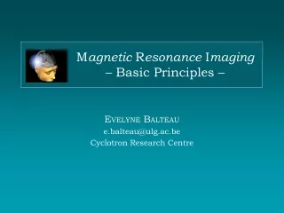
1. Magnetic Resonance Imaging– Basic Principles – EVELYNE BALTEAU e.balteau@ulg.ac.be Cyclotron Research Centre

2. Overview • Brief history of MRI • Magnetic properties of the nuclei • Interaction with B0 • Interaction with B1 • Relaxation • Signal Localization • Contrast

3. 1940 1950 1960 1970 1980 1990 2000 index Brief history of MRI 1971 – Damadian : NMR used to distinguish healthy and malignant tissues  medical application but imaging technique… 1946 – Bloch & Purcell independently describe the NMR phenomenon 1973 – Lauterbur : Back-projection MRImaging 1952 – Bloch & Purcell Nobel Prize in Physics 1975 – Ernst : Fourier Transform based MRI (demonstrated by Edelstein in 1980) 1977 – Mansfield : Echo-Planar Imaging NMR developed as analytical tool (no medical application) 1990 – Ogawa : functional MRI (BOLD) 1991 – Ernst Nobel Prize in Chemistry 2003 – Lauterbur & Mansfield Nobel Prize in Medicine

4. External magnetic field B0 = 3 T Magnetic properties of the NUCLEI Electromagnetic field B1(Radio-frequency or RF) index MRI : magnetic stuff !! 60000  the earth’s magnetic field !!!! FM radio-waves : 88.8 – 108.8 MHz !!

5. Nuclear MRI  no radioactivity !!  nucleus is like a small magnet The nuclear SPIN  characterized by a spin number I  quantum mechanics !!  a nucleus with I 0 behaves like a small magnet index Magnetic properties of the nuclei The Hydrogen nucleus  the most abundant (~⅔ of the atoms in living tissues)

6. index Behaviour of the nuclei interacting with : 1. The external magnetic field B0 • Equilibrium state 2. The electromagnetic field B1 (RF) • Disturbance

7. index Interaction with B0 1. Orientation :

8. index Interaction with B0 2. Energy states : DE = għBo = ħwo

9. index Interaction with B0 3. Precession :  Rotation or precession about the axis of the magnetic field Bo with frequency : wo =gBo wo =Larmor frequency g =gyromagnetic ratio

10. y x index Interaction with B0 3. Precession : At the equilibrium state : - rotation in phase - no transverse magnetization Mxy

11. index Interaction with B0 4. Summary : at the equilibrium state : 1. spin orientation « up » > « down »  longitudinal magnetization Mz 2. precession  no transverse magnetization Mxy

12. TRANSITIONS REPHASING Transitions E1  E2  Mz decreases Phase coherence increases Mxy increases index Interaction with B1Resonance phenomenon !!! RF frequency = Larmor frequency = w0 !!!

13. index Interaction with B1 From the macroscopic point of view… Two different processes : 1. Transitions E1  E2  Mzdecreases 2. Rephasing  Mxyincreases  The macroscopic magnetization flips from the z-axis to the xy-plane and precesses

14. TRANSITIONS DEPHASING Transitions E2  E1  Mz increases  T1 relaxation Dephasing  Mxy decreases  T2 relaxation index Relaxation  back to the equilibrium state…

15. index Relaxation  back to the equilibrium state… Two different processes : 1. Transitions E2  E1  Mz increases  T1 relaxation 2. Dephasing  Mxy decreases  T2 (exponential) relaxation Free Induction Decay :  received signal !!  informations from the tissues of interest

16. index Signal localization Up to now : the signal received contains information from the entire body !! Not interesting !  Use field gradients to spatially encode the signal Three steps : 1. Slice selection slice = matrix 2. Frequency-encoding columns 3. Phase-encoding lines

17. index Signal localization 1. Slice selection gradient Resonance Phenomenon : wRF = wo !!! Before Gz is applied : all the spins precess with the same Larmor frequency wo  all could resonate !! During application of Gz : the spins precess with  w  only spins with frequency = wRF resonate

18. index Signal localization 2. Frequency-encoding gradient Slice selection : but still no spatial discrimination within the slice ! Before Gx is applied : all the spins precess with the same Larmor frequency wo During application of Gx : the spins precess with  frequencies  Fourier Transform of the signal allows discrimination between columns !

19. index Signal localization 3. Phase-encoding gradient Before Gy is applied : all the spins precess with the same Larmor frequency wo During application of Gy : the spins precess with  frequencies  induces phase difference between the lines After application of Gx : all the spins precess again at the same Larmor frequency, but with different phase shifts from line to line…

20. index Contrast in MRI Grey-level images :  the intensity of a voxel depends on the intensity of the corresponding signal.

21. index Contrast in MRI

22. index Contrast in MRI  Contrast depends on : 1. tissue properties : T1, T2, r user-independent 2. sequence parameters : TR, TE, … TR = repetition time = time interval between two RF pulses TE = echo time = when the acquisition is performed user-dependent

23. index Contrast in MRI Sequence parameters : TR and TE

24. index Contrast in MRI T2-weighted image : long TR – long TE

25. TR = 3370 ms TE = 112 ms CSF GM WM index Contrast in MRI T2-weighted image : long TR – long TE

26. index Contrast in MRI T1-weighted image : short TR – short TE

27. TR ~ 500 ms TE ~ 10 ms WM GM CSF index Contrast in MRI T1-weighted image : short TR – short TE

28. index Contrast in MRI Illustration : une pomme dans un verre d’eau… Contraste en T1 – TE court et TR variable Cas d’une impulsion RF initiale de 90°

29. index Contrast in MRI Illustration : une pomme dans un verre d’eau… Contraste en T1 – TE court et TR variable Cas d’une impulsion RF initiale de 180°

30. index Contrast in MRI Illustration : une pomme dans un verre d’eau… Contraste en T2 – TR long et TE variable (Impulsion RF initiale de 90°)

31. The 3.0 Tesla Allegra MR scanner at the Cyclotron Research Centre

32. The 3.0 Tesla Allegra MR scanner at the Cyclotron Research Centre

33. The 3.0 Tesla Allegra MR scanner at the Cyclotron Research Centre

34. index