Download
1 / 23
230 likes | 465 Vues
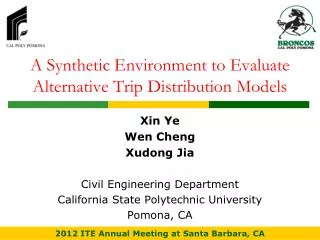
A Synthetic Environment to Evaluate Alternative Trip Distribution Models. Xin Ye Wen Cheng Xudong Jia Civil Engineering Department California State Polytechnic University Pomona, CA. 2012 ITE Annual Meeting at Santa Barbara, CA. Alternative Trip Distribution Models.

E N D
A Synthetic Environment to Evaluate Alternative Trip Distribution Models Xin Ye Wen Cheng XudongJia Civil Engineering Department California State Polytechnic University Pomona, CA 2012 ITE Annual Meeting at Santa Barbara, CA
Alternative Trip Distribution Models • Importance of trip distribution models • Gravity model (1950’) • Singly- and doubly-constraint • Entropy maximization • TAZ level • Destination choice model (1970’) • Utility maximization • Individual level Cal Poly Pomona Civil Engineering Department
Comparisons of Gravity Model (GM) and Destination Choice Model (DCM) • Similarity: • Wilson (1967): destination choice and singly-constraint gravity models have the same mathematical formula • Then, what is the difference? Cal Poly Pomona Civil Engineering Department
Difference between GM and DCM • TAZ level vs. Individual level • Can GM not differentiate market segments? • DCM still applied at TAZ level • Trip-end survey for trip attraction models • Is GM a subset of DCM?
Objectives of This Study • To provide a better understanding of difference and similarity between GM and DCM • To introduce the research method of using synthetic environment • To visualize spatial aggregation errors in DCM Cal Poly Pomona Civil Engineering Department
Research Method [1]:Limitations of Using Real Data • True trip matrices are not known • Imperfect indirect measurement (average trip length, trip length distribution, aggregated trip matrices, etc.) • Imperfect input data for TAZ/Network • Survey sampling may not be perfectly random • Travelers may not really maximize utility Cal Poly Pomona Civil Engineering Department
Research Method [2]: Advantages of Synthetic Environment • Perfect input data for TAZ/Network • Assume travelers to maximize utility • Trip matrices are known and can be aggregated to any spatial levels • Survey sampling can be perfectly random Cal Poly Pomona Civil Engineering Department
Synthesized City • A city of square shape and its side length is 20 miles • Total population is about 500,000 and Total employees is about 250,000 • The city is divided into 200×200 uniform square cells and each cell’s side length is 0.1 miles • Cell is the smallest spatial unit for allocating trip’s OD, residents’ homes and employees’ jobs • Each cell is located by the x-y coordinates of its geometric center
Transportation Network • A grid-like transportation network Cal Poly Pomona Civil Engineering Department
Spatial Distributions of Population and Employees • Use probability density functions of mixed bivariate normal distribution to distribute population/employees Cal Poly Pomona Civil Engineering Department
Spatial Distribution of Population Cal Poly Pomona Civil Engineering Department
Spatial Distribution of Employees Cal Poly Pomona Civil Engineering Department
Travel Synthesis • Each person makes one trip from home cell to another cell • Calculate utilities and choose the cell with the maximum utility as destination cell Cal Poly Pomona Civil Engineering Department
Model Developments • Aggregate cells to TAZs • 200 × 200 cells aggregated 20 × 20 TAZs • Side length of TAZ is 1 mile • Household travel survey • 1% of population are sampled to report their destination cell (sample size ≈ 5,000) • Destination choice model • Develop the model at TAZ level • Maximize the log-likelihood function • Gravity model • Estimate linear regression model for trip attraction • Adjust parameter for friction factors to match the trip length distribution from the survey
Destination Choice Models Average trip length of short-distance trip: 1.84 Miles Average trip length of long-distance trip: 5.02 Miles
Gravity Models Long Trip Short Trip
Comparisons of Model Applications [1]: Trip Matrices Cal Poly Pomona Civil Engineering Department
Comparisons of Model Applications [2]: Trip Attractions Cal Poly Pomona Civil Engineering Department
Conclusions [1] • Gravity model: • Linear regression model does not provide consistent coefficients for trip attraction variables • Conventional method to calibrate friction factors can provide consistent coefficient for travel impedance • Destination choice model: • When the average trip length is much larger than the TAZ size, coefficients and estimated trip matrices are reasonable • When the average trip length is closer to TAZ size, coefficients and estimated trip matrices are biased Cal Poly Pomona Civil Engineering Department
Conclusions [2] • Observed trip length distribution may not be perfectly matched in a reasonable trip distribution model at aggregate level Cal Poly Pomona Civil Engineering Department


![[Alternative Ownership Models]](https://cdn2.slideserve.com/5345939/alternative-ownership-models-dt.jpg)