Download

1 / 32
341 likes | 748 Vues
Atomic Line Emission Spectra and Niels Bohr. Bohr is credited with the first modern model of the hydrogen atom based on the “ line spectra ” of atomic emission sources. He proposed a “ planetary ” structure for the atom where the electrons circled the nucleus in defined orbits.

E N D
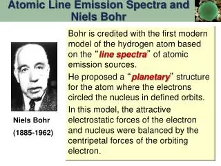
Atomic Line Emission Spectra and Niels Bohr Bohr is credited with the first modern model of the hydrogen atom based on the “line spectra” of atomic emission sources. He proposed a “planetary” structure for the atom where the electrons circled the nucleus in defined orbits. In this model, the attractive electrostatic forces of the electron and nucleus were balanced by the centripetal forces of the orbiting electron. Niels Bohr (1885-1962)
Spectrum of White Light When white light passes through a prism, all the colors of the rainbow are observed.
Spectrum of Excited Hydrogen Gas When the light from a discharge tube containing a pure element (hydrogen in this case) is passed through the same prism, only certain colors (lines) are observed. Recall that color (wavelength) is related to energy via Planck’s law.
Line Emission Spectra of Excited Atoms • Excited atoms emit light of only certain wavelengths • The wavelengths of emitted light are unique to each individual element.
Line Spectra of Other Elements • Each element has a unique line spectrumof colors it emits when heated to the point of glowing.
Atomic Spectra & Bohr Model + Bohr asserted that line spectra of elements indicated that the electrons were confined to specific energy states calledorbits. The orbits or energy levels are “quantized” such that only certain levels are allowed. n = 1, 2, 3...
Atomic Spectra & Bohr Model + Bohr asserted that line spectra of elements indicated that the electrons were confined to specific energy states calledorbits. The lines (colors) corresponded to “jumps” or transitions between the levels.
Origin of Line Spectra The “Balmer” series for the hydrogen atom is in the visible region of the spectrum. A “series” of transitions end with a common lower level.
Wave or Quantum Mechanics • Irwin Schrödinger proposed that matter can be described as a wave. • An electron is described by a Wave Function “” that completely defines a system of matter. E. Schrodinger 1887-1961
Types of Orbitals • The solutions to the Schrödinger equation yields the probability in 3-dimensons for the likelihood of finding and electron about the nucleus. • It is these probability functions that give rise to the familiar hydrogen-like orbitals that electrons occupy.
Quantum Numbers & Electron Orbitals Quantum Numbersare terms that arise from the mathematics of the Schrödinger equation. They describe location of an electron in a particular orbital much like an address. Each electron in an orbital has its own set of three quantum numbers. “n” = 1, 2, 3, 4…. Principal Quantum Number shell Azimuthal or Angular Quantum Number “L” = 0, 1, 2, 3…” sub-shell Magnetic Quantum Number “ml” ml may take on the value an integer from – l to + l individual orbitals
Quantum Numbers & Electron Orbitals Each “l” within an “n-level” represents a sub-shell. Each “l” sub-shell is divided into ml degenerate orbitals, where mldesignates the spatial orientation of each orbital. Type of orbital # of orbitals l = 0 “s” sub-shell (sharp) 1 l = 1 “p” sub-shell (Principal) 3 l = 2 “d” sub-shell (diffuse) 5 l = 3 “f” sub-shell (fine) 7 each subshell contains 2l+1 orbitals
Types of Orbitals s orbital p orbital d orbital
s-Orbitals • l = 0, ml = 0 • 2l+1 = 1 • one s-orbital that extends in a radial manner from the nucleus forming a spherical shape.
Spherical Nodes 2 s orbital • All s-orbitals have “n-1” spherical nodes. • A 1s-orbital has none, a 2s has 1 and so on. • These nodes represent a sphere of zero probability for finding an electron
p-Orbitals When n = 2, then l = 0 and 1 Therefore, in 2nd shell there are 2 types of orbitals, i.e. 2 sub-shells For l = 0 ml = 0 (s-orbital) For l = 1 ml = -1, 0, +1 2(1) + 1 or 3 p-orbitals Each p-orbital is characterized by a “nodal plan”
p-Orbitals The three degenerate p-orbitals spread out on the x, y & z axis, 90° apart in space.
d-Orbitals When n = 3, l = 0, 1, 2 resulting in 3 sub-shells within the shell. For l = 0, ml = 0 s-sub-shell with a single s-orbital For l = 1, ml = -1, 0, +1 p-sub-shell with 3 p-orbitals For l = 2, ml = -2, -1, 0, +1, +2 d-sub-shell with 5 d-orbitals 2(2)+1 = 5
d-Orbitals s-orbitals have no nodal planes (l = 0) p-orbitals have one nodal plane (l = 1) d-orbitals therefore have two nodal planes (l = 2)
f-Orbitals When n = 4, l = 0, 1, 2 & 3 resulting in 4 sub-shells within the shell. For l = 0, ml = 0 s-sub-shell with a single s-orbital For l = 1, ms = -1, 0, +1 p-sub-shell with 3 p-orbitals For l = 2, ms = -2, -1, 0, +1, +2 d-sub-shell with 5 d-orbitals For l = 3, ms = -3, -2, -1, 0, +1, +2, +3 f-sub-shell with 7 f-orbitals 2(3)+1 = 7
f-Orbitals All have 3 nodal planes. One of the 7 possible f-orbitals.
Arrangement of Electrons in Atoms • Each orbital can accommodate no more than 2 electrons • Since each electron is unique, we need a way to distinguish the individual electrons in an orbital from one another. • This is done via the 4th quantum number, “ms”.
Electron Spin N S When an atom with one unpaired electron is passed through a magnetic field, the path is altered into two directions. Detector Source of electrons This means that the electrons have a magnetic moment!
Electron Spin Since there were 2 pathways in the experiment, there must be 2 spins affected by the magnetic field. One spinning to the right, one spinning to the left. Each “spin state” is assigned a quantum number ms = ± ½ + ½ for “spin up” ½ for “spin down”
Electron Spin Quantum Number, ms Electron Spin The experiment results indicate that electron has an intrinsic property referred to as “spin.” Two spin directions are given by ms where ms = +1/2 and -1/2.
Electron Spin & Magnetism • Diamagnetic Substances: Are NOT attracted to a magnetic field • Paramagnetic Substances: ARE attracted to a magnetic field. • Substances with unpairedelectrons are paramagnetic.
Measuring Paramagnetism When a substance containing unpaired electrons is place into a magnetic field, it is attracted to that magnetic field. The effect is proportional to the number of unpaired electrons.
Electron Quantum Numbers Principal (n) shells n = 1, 2, 3, 4, ... Angular (l) sub-shells l = 0, 1, 2, ... n - 1 Magnetic (ml) orbitals ml = - l ... 0 ... + l Spin (ms) individual electrons ms = ½ The Pauli Exclusion Principle: Every electron in an atom has a unique set of 4 quantum #s.