Download
1 / 69
690 likes | 845 Vues
Relationships between Land Cover and Spatial Statistical Compression in High-Resolution Imagery. James A. Shine 1 and Daniel B. Carr 2 34 th Symposium on the Interface 19 April 2002 1 George Mason University & US Army Topographic Engineering Center 2 George Mason University.

E N D
Relationships between Land Cover and Spatial Statistical Compressionin High-Resolution Imagery James A. Shine1 and Daniel B. Carr2 34th Symposium on the Interface 19 April 2002 1 George Mason University & US Army Topographic Engineering Center 2 George Mason University
Outline of Talk • The Variogram • Motivation and Procedure • Past Results • Present Results • Analysis and Conclusions • Future Work
Spatial Statistics: The Variogram -A plot of average variance between points vs. distance between those points (L2) -If data are spatially uncorrelated, get a straight line -If data are spatially correlated, variance generally increases with distance -Directional component also a consideration (N-S, E-W, omnidirectional)
Typical image variogram (left), Important quantities (right)
Variogram Applications -Determination of range for sampling applications: ground truth supervised classification -Model for estimation/prediction applications (forms of kriging)
Outline of Talk • The Variogram • Motivation and Procedure • Past Results • Present Results • Analysis and Conclusions • Future Work
MOTIVATION Large data sets, computational challenges (10^6-10^7 data points per km^2 at 1 m resolution for pixels) Large computation times not conducive to real-world applications such as rapid mapping Compression will reduce computation time, But how much can we reduce without losing information?
PROCEDURE Transfer data from imagery to text file Compute variograms (FORTRAN code) Format and plot the variograms Compare variograms with full data sets vs variograms with reduced data sets
Imagery Ft. A.P. Hill, Ft. Story (both in Virginia) : 1-meter resolution, 4-band CAMIS imagery, collected by US Army Topographic Engineering Center (TEC) Others: 4-meter resolution, 4-band IKONOS imagery, obtained from TEC’s imagery library and also commercially available. Bands: 1. Blue (~450 nm) 2. Green (~550 nm) 3. Red (~650 nm) 4. Near Infrared (~850 nm)
Outline of Talk • The Variogram • Motivation and Procedure • Past Results • Present Results • Analysis and Conclusions • Future Work
Previous Results: Ft. A.P. Hill, VA (Shine, Interface 2001) Mostly forest, some manmade 2196 x 2016=4.4x10^6 pixels
Compression works well for AP Hill imagery; Band 1 (blue) variograms shown below
Other A.P. Hill bands also compressed well: Band 2 (Green), N-S at right, E-W bottom left, Average bottom right
Band 3 (Red), N-S at right, E-W bottom left, Average bottom right
Band 4 (IR), N-S at right, E-W bottom left, Average bottom right
Outline of Talk • The Variogram • Motivation and Procedure • Past Results • Present Results • Analysis and Conclusions • Future Work
Fort Story, VA results completed, Plus some new imagery: New York City Ft. Stewart, GA Ft. Moody, GA Wright-Patterson AFB, OH Ft. Huachuca, AZ
Fort Story, VA New York City Ft. Stewart, GA Ft. Moody, GA Wright-Patterson AFB, OH Ft. Huachuca, AZ
Original Ft. Story image: Water, forest, urban 3999x4999= 2.0x10^7 pixels
Ft. Story,original Band One (Blue) N-S at right, E-W bottom left, Average bottom right
Ft. Story,original Band Two(Green) N-S at right, E-W bottom left
Ft. Story Results -Full variogram is very smooth (exponential/spherical), but compression is not good; compressed variogram significantly different from full variogram -Why does AP Hill compress well and Story does not? Could be losing a level on a nested model (right), but perhaps different landcover or terrain reacts differently to compression. -Need to compare different types of imagery and hopefully make some inferences
Subarea from Ft. Story: just forest 524x408=2.1x10^5 pixels
Ft. Story forest subimage Band One (Blue) N-S at right, E-W bottom left Average bottom right
Ft. Story forest subimage results -Variograms seem to be unbounded (linear) -Compression matches original pretty well, much better than for the full image -Do some more tests with other images and landcovers
New Results: Fort Story, VA New York City Ft. Stewart, GA Ft. Moody, GA Wright-Patterson AFB, OH Ft. Huachuca, AZ
New York City 2000 x 2000 Urban, water, smoke (9/12/01)
New York City Blue E-W, N-S, average
New York City Green E-W, N-S, average
New York City Results -Variogram seems unbounded (linear) -Almost no difference between the full and compressed variograms
New Results: Fort Story, VA New York City Ft. Stewart, GA Ft. Moody, GA Wright-Patterson AFB, OH Ft. Huachuca, AZ
Fort Stewart Mostly fields 2559x2559= 6.5x10^6 pixels
Ft. Stewart Blue E-W, N-S, average
Ft. Stewart Green E-W, N-S, average
Ft. Stewart Red E-W, N-S, average
Ft. Stewart IR E-W, N-S, average
Ft. Stewart Results -Full variogram is very smooth (exponential/spherical) -Almost no difference between full and compressed variograms, except very slightly in Blue band
New Results: Fort Story, VA New York City Ft. Stewart, GA Ft. Moody, GA Wright-Patterson AFB, OH Ft. Huachuca, AZ
Ft. Moody fields 1202x1742= 2.1x10^6 pixels
Ft. Moody fields Blue E-W, N-S, average
Ft. Moody fields Green E-W, N-S, average
Ft. Moody fields Red E-W, N-S, average
Ft. Moody fields IR E-W, N-S, average
Ft. Moody forest 1325x1767= 2.3x10^6 pixels
Ft. Moody forest , Blue , E-W (no spatial dependence after 3 pixels, so compression is useless; all bands and directions give same non-dependence)
Ft. Moody Results • Field subset variogram is mixed: mostly linear in visible bands, mostly spherical/exponential in IR band. Compresses well although compressed variogram is greater in magnitude than full variogram for the Blue and Green bands • Forest subset shows no spatial dependence, compression is irrelevant
New Results: Fort Story, VA New York City Ft. Stewart, GA Ft. Moody, GA Wright-Patterson AFB, OH Ft. Huachuca, AZ
Wright-Patterson AFB, Ohio mostly fields, some urban 1385x1692=2.3x10^6 pixels