Download
1 / 13
170 likes | 386 Vues
Study on Dispersion Compensating Fiber. Presented by Rajkumar Modak (2011PHS7184) Suvayan Saha (2011PHS7099). Under the Guidance of Prof. B.P. Pal Dr. R.K. Varshney. Ref: Google Images. Work Plan.

E N D
Study on Dispersion Compensating Fiber Presented by RajkumarModak (2011PHS7184) SuvayanSaha (2011PHS7099) Under the Guidance of Prof. B.P. Pal Dr. R.K. Varshney Ref: Google Images
Work Plan • Study on dispersion compensating fiber. • Study on Simple single cored DCF. • Study on coaxial index guiding DCF. • Study on micro structured DCF.
Motivation • In conventional fibers • Minimum attenuation is at 1.55 μm. • Dispersion is positive at 1.55 μm , i.e. 17-20 ps/km-nm. • To send large no. of data within a pulse in a fiber. • Decreases the dispersion. • Two choices • Design a fiber with low dispersion at 1.55 μm. • Add another fiber with negative dispersion. .
Basic principle where = material dispersion coefficient = waveguide dispersion coefficient = effective index at propagating wavelength = propagating wavelength. • To achieve zero dispersion where and are the lengths of SMF & DCF. Ref: Ghatak & Thyagarajan - Introduction to fiber optics, chapter 15
Methodology • Matrix formulation: ; where , = , = guided wavelength The solution for j th region is, Boundary conditions at j th & j+1 gives the matrix where an arbitrary variation of is replaced by a large number of steps Ref: Ghatak & Thyagrajan – Introduction to fiber optics , chapter-25
verification of matrix method For single modes at = 1 µm. Fig-2(b) n1=1.503,n2=1.500,d1=4 µm.,d2=4 µm. Fig-2(a) calculated b = 0.53184 ( result according to book=0.53177) Fig-3(a)Fig. 3(b): n1=1.503,n2=1.500,d1=12µm,d2=4µm,d3=µm calculated b = 0.5312(result according to book= 0.5312) Ref: Ghatak & Thyagrajan – Introduction to fiber optics , chapter-25
For double modes at = .5 µm. Fig-4(a) Fig-4(b) n1=1.503,n2=1.5,d1=12µm,d2=4µm,d3=µm Fig-5(c) Fig-5(d) calculated b= 0.2381 (result according to book = 0.2379) calculated b= 0.7896 (result according to book = 0.78959) Ref: Ghatak & Thyagrajan – Introduction to fiber optics , chapter-25
Optical fiber system • Cylindrically symmetric step index fiber : = core refractive index = cladding refractive index • For fibers the concept of matrix treatments are same, just the wave function is replaced by for core for cladding Ref: Ghatak & Thyagararan - Introduction to fiber optics, chapter 24 .
Determination of wavelength dependence of refractive index. • Wavelength dependence of the refractive index for silica is given by Sellemeier Equation, where = operating wavelength , are known as Sellemeier coefficients . • Concentration of germanium is related with the refractive indices as: where = refractive index of pure silica, n = refractive index at a given wavelength, are constants at particular wavelength. • The refractive index for any arbitrary concentration is given by where are constants at particular wavelength. • Ref :- A. K. Ghatak, I. C. Goyal, R. K. Varshney – “Fiber Optica”, chapter 3
Fig. 6(a) Fig. 6(b) Fig. 7(a) Fig. 7(b) • Ref: 1. Ghatak & Thyagarajan-Introduction to fiber optics, chapter 15, • K. Thyagarajan, B. P. Pal, “Modelling dispersion in optical fibers: applications to dispersion tailoring and dispersion compensation”, Journal of Opt. FiberCommun. Rep. , vol. 4, 2007, pp. 1- 42
Δ=2%, =1.4729004, =1.44402 a=1μm D= -577.12252 ps/km-nm Fig. 7 Fig. 8 • Ref: 1. Ghatak & Thyagarajan-Introduction to fiber optics, chapter 15, • K. Thyagarajan, R. K. Varshney, P. Palai, A. K. Ghatak and I. C. Goyal, “A Novel Design of a Dispersion Compensating Fiber ” , IEEE Photon. Tech. Letts. , vol. 8, no. 11, novenber 1996, pp. 1510-1512.
REFERENCES • Ajoy Ghatak & K. Thyagarajan – “Introduction to fiber optics” (First south asian edition 1999, reprinted 2011 ), Chapter 15 and Chapter 24. • K. Thyagarajan, R. K. Varshney, P. Palai, A. K. Ghatak and I. C. Goyal, “A Novel Design of a Dispersion Compensating Fiber ” , IEEE Photon. Tech. Letts. , vol. 8, no. 11, novenber 1996, pp. 1510-1512. • A. K. Ghatak, I. C. Goyal, R. K. Varshney – “Fiber Optica”, Chapter 3 • A. K. Ghatak, A. Sharma, R. Tewari – “Understanding Fiber Optics on PC ” , Chapter-2, 4, 8, 13. • K. Thyagarajan, B. P. Pal, “Modelling dispersion in optical fibers: applications to dispersion tailoring and dispersion compensation”, Journal of Opt. Fiber Commun. Rep. , vol. 4, 2007, pp. 1- 42 • M. R. Shenoy , K. Thyagarajan and A. K. Ghatak , “Numerical Analysis of Optical Fibers Using Matrix Approach”, Journal of Lightwave Tech. vol. 6, no. 8, Aug. 1988.