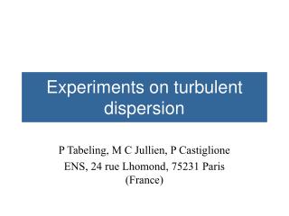
Experiments on turbulent dispersion
This study explores turbulent dispersion through experiments conducted under varying velocity field conditions. We detail dispersion mechanics within smooth and rough fields, following the Batchelor regime and the inverse cascade principles. Significant theoretical advancements, particularly the resolution of the Kraichnan model, have enriched our understanding since the 20th century. Our experiments capture high-order statistics, Lagrangian properties, and scalar spectra, revealing insights into concentration dynamics and the role of energy spectra. Results validate the theoretical framework linking turbulence and dispersion.

Experiments on turbulent dispersion
E N D
Presentation Transcript
Experiments on turbulent dispersion P Tabeling, M C Jullien, P Castiglione ENS, 24 rue Lhomond, 75231 Paris (France)
Outline • 1 - Dispersion in a smooth field (Batchelor regime) • 2 - Dispersion in a rough field (the inverse cascade)
Important theoretical results have been obtained in the fifties, sixties, (KOC theory, Batchelor regime,.. ) In the last ten years, theory has made important progress for the case of rough velocity fields essentially after the Kraichnan model (1968) was rigorously solved (in 1995 by two groups) In the meantime, the case of smooth velocity fields, called the Batchelor regime, has been solved analytically.
Experiments on turbulent dispersion have been performed since 1950, leading to important observations such as scalar spectra, scalar fronts,... - However, up to recent years no detailed : - Investigation of lagrangian properties, pair or multipoint statistics - Reliable measurement of high order statistics In the last years, much progress has been done
Principle of the experiment B I U 2 fluid layers, salt and Clear water Magnet
The experimental set-up 15 cm 5- 8 mm
Is the flow we produce this way two-dimensional ? - Stratification accurately suppresses the vertical component (measured as less than 3 percents of the horizontal component) - The velocity profile across the layer is parabolic at all times and quickly returns to this state if perturbed (the time constant has been measured to be on the order of 0.2s) - Under these circumstances, the equations governing the flow are 2D Navier Stokes equations + a linear friction term - Systematic comparison with 2D DNS brings evidence the system behaves as a two-dimensional system
Velocity profile for two components, along a line
U smooth - U can be expanded in Taylor series everywhere (almost) - The statistical statement is : (called structure function of order 2) This situation gives rise to the Batchelor regime U rough Structure functions behave as
A way to know whether a velocity field is smooth or rough, is to inspect the energy spectrum E(k) If b < 3 then the field is rough If b > 3 then the field is smooth This is equivalent to examining the velocity structure function, For which the boundary between rough and smooth is a=1
CHARACTERISTICS OF THE VELOCITY FIELD (GIVING RISE TO BATCHELOR REGIME) Energy Spectrum 2D Energy spectrum
RELEASING THE TRACER Drop of a mixture of fluorescein delicately released on the free surface
CHARACTERIZING THE BATCHELOR REGIME There exists a range of time in which statistical properties are stationary
Turbulence deals with dissipation : something is injected at large scales and ‘ burned ’ at small scales; in between there is a self similar range of scales called « cascade » The rule holds for tracers : the dissipation is In a steady state, c is a constant
TWO WORDS ON SPECTRA... The spectrum Ec(k) is related to the Fourier decomposition of the field Its physical meaning can be viewed through the relation They are a bit old-fashioned but still very useful
SPECTRUM OF THE CONCENTRATION FIELD 2D Spectrum
C=1 C=0 r Does the k -1 spectrum contain much information ?
GOING FURTHER…. HIGHER ORDER MOMENTS In turbulence, the statistics is not determined by the second order moment only (even if, from the practical viewpoint, this may be often sufficient) Higher moments are worth being considered, to test theories, and to better characterize the phenomenon.
A central quantity : Probability distribution function (PDF) of the increments The pdf of DCr is called : P(DCr) r C2 C1
Taking the increment across a distance r amounts to apply a pass-band filter, centered on r. DCr r
Two pdfs, at small and large scale PDF for r = 0.9 cm PDF for r = 11 cm
PDF OF THE INCREMENTS OF CONCENTRATION IN THE SELF SIMILAR RANGE
Structure functions The structure function of order p is the pth-moment of the pdf of the increment
STRUCTURE FUNCTIONS OF THE CONCENTRATION INCREMENTS
DO WE UNDERSTAND THESE OBSERVATIONS ? TO UNDERSTAND = SHOW THE OBSERVATIONS CAN BE INFERRED FROM THE DIFFUSION ADVECTION EQUATIONS The answer is essentially YES, after the work by Chertkov, Falkovitch, Kolokolov, Lebedev, Phys Rev E54,5609 (1995) - k-1Spectrum - Exponential tails for the pdfs - Logarithmic like behaviour for the structure functions
CONCLUSION : THEORY AGREES WITH EXPERIMENT A PIECE OF UNDERSTANDING, CONFIRMED BY THE EXPERIMENT, IS OBTAINED
The life of a pair of particles released in the system How two particles separate ? exponentially, according to the theory
Separation (squared) for100000 pairs LINEAR LINEAR LOG-LINEAR C Jullien (2001)
Part 2 :DISPERSION IN THE INVERSE CASCADE
Reminding... • We are dealing with a diffusion advection given by : Two cases : u(x,t) smooth u(x,t) rough
l e 2l 4l Cartoon of the inverse cascade in 2D
vorticity streamfunction
Energy spectrum for the inverse cascade 2D spectrum Slope -5/3 injection dissipation
Averaged squared separation with time in the inverse cascade Slope 3
Why the pairs do not simply diffuse ? li Central limit theorem : the squared separation grows as t2
Lagrangian distributions of the separations t=10 s t=1s