Download
1 / 14
140 likes | 290 Vues
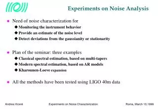
Experiments on Noise Analysis. Need of noise characterization for Monitoring the instrument behavior Provide an estimate of the noise level Detect deviations from the gaussianity or stationarity Plan of the seminar: three examples Classical spectral estimation, based on multi-tapers

E N D
Experiments on Noise Analysis • Need of noise characterization for • Monitoring the instrument behavior • Provide an estimate of the noise level • Detect deviations from the gaussianity or stationarity • Plan of the seminar: three examples • Classical spectral estimation, based on multi-tapers • Modern spectral estimation, based on AR models • Kharounen-Loeve expansion • All the methods have been tested using LIGO 40m data
Multi-tapering in one slide • Purpose: control both bias and variance of a spectral estimate, over a finite sample. • Perform several spectral estimates with different windows, and average. • Choose the windows so as to be “orthogonal”, at fixed frequency resolution. • Use the so called Discrete Prolate Spheroidal Sequences
A typical noise spectrum (LIGO 40m) • Wideband • Narrow spectral features • Physical resonances • Harmonics of the line • Need to monitor the spectrum over time.
Comparison of spectral estimates (1) • The Hamming window gives the best resolution. • Lower variance from the multi-taper estimate • Better choice: adapt the coefficients of the different tapers. • Warning: this is actually an harmonic of the 60 Hz line!
Comparison of spectral estimates (2) • The use of several different windows is possible only reducing the frequency resolution: NumTapers <= N • The f.r. is necessarily more limited, as at the 300 Hz line. • Adapting the tapers helps off-resonance.
Modern spectral estimates • Model the noise as gaussian noise filtered through a linear model. • Estimate the model parameters. • Choose the model order on the basis of the final prediction error.
Low order models • The FPE criterion is not robust enough: it is not sensitive to the narrow spectral features. • The suggested order is definitely too small.
Higher order models • Increasing the order the narrow features are resolved. • Monitoring the values of the coefficients, that is the zeros (and poles, for ARMA models) one can detect non-stationarities. • But: some of the lines are actually discrete components of the spectrum.
Karhounen-Loeve basis • Spectral estimates rely on the statistical independence of the different lines • The KL basis gives statistically independent coefficients also over short samples.
Eigenvalues and RMS noise • The basis elements are the eigenvectors of the correlation matrix R. • The eigenvalues measure how each component contributes to the RMS noise.
KL as a selector of spectral features • Each KL element actually corresponds to some spectral feature. • They are ordered on the basis of the relative RMS “importance.”
Coefficient monitoring (1) • Pairs of KL basis elements correspond to the same eigenvalue • Coefficients estimated from different samples are uncorrelated and gaussianly distributed. • In other languages they correspond to the Principal Components of the noise spectrum
Coefficient monitoring (2) • Elements of the discrete part of the spectrum (infinitely narrow lines) appear much differently • In a scatter plot they manifest perfect correlation, and their relative fase remains correlated in time. • Without surprise, this component corresponds to an harmonic of the line.
Coefficient monitoring (3) • Deviations from the predicted model may signal a change of noise level in the specific component. • In the specific example, the damping out of a resonance possibly excited by the lock acquisition.