Audio Signal Processing -- Quantization
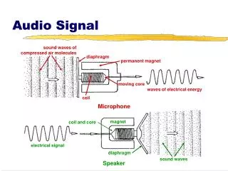
Audio Signal Processing -- Quantization. Shyh-Kang Jeng Department of Electrical Engineering/ Graduate Institute of Communication Engineering. Overview. Audio signals are typically continuous-time and continuous-amplitude in nature

Audio Signal Processing -- Quantization
E N D
Presentation Transcript
Audio Signal Processing-- Quantization Shyh-Kang Jeng Department of Electrical Engineering/ Graduate Institute of Communication Engineering
Overview • Audio signals are typically continuous-time and continuous-amplitude in nature • Sampling allows for a discrete-time representation of audio signals • Amplitude quantization is also needed to complete the digitization process • Quantization determines how much distortion is presented in the digital signal
Binary Numbers • Decimal notation • Symbols: 0, 1, 2, 3, 4, …, 9 • e.g., • Binary notation • Symbols: 0, 1 • e.g.,
Negative Numbers • Folded binary • Use the highest order bit as an indicator of sign • Two’s complement • Follows the highest positive number with the lowest negative • e.g., 3 bits, • We use folded binary notation when we need to represent negative numbers
Quantization Mapping • Quantization • Dequantization Continuous values Binary codes Binary codes Continuous values
Quantization Mapping (cont.) • Symmetric quantizers • Equal number of levels (codes) for positive and negative numbers • Midrise and midread quantizers
Uniform Quantization • Equally sized range of input amplitudes are mapped onto each code • Midrise or midread • Maximum non-overload input value, • Size of input range per R-bit code, • Midrise • Midread • Let
1.0 1.0 3/4 01 00 1/4 0.0 10 -1/4 -3/4 11 -1.0 -1.0 2-Bit Uniform Midrise Quantizer
Uniform Midrise Quantizer • Quantize: code(number) = [s][|code|] • Dequantize: number(code) = sign*|number|
2-Bit Uniform Midtread Quantizer 1.0 1.0 2/3 01 00/ 10 0.0 0.0 11 -2/3 -1.0 -1.0
Uniform Midread Quantizer • Quantize: code(number) = [s][|code|] • Dequantize: number(code) = sign*|number|
Two Quantization Methods • Uniform quantization • Constant limit on absolute round-off error • Poor performance on SNR at low input power • Floating point quantization • Some bits for an exponent • the rest for an mantissa • SNR is determined by the number of mantissa bits and remain roughly constant • Gives up accuracy for high signals but gains much greater accuracy for low signals
Floating Point Quantization • Number of scale factor (exponent) bits : Rs • Number of mantissa bits: Rm • Low inputs • Roughly equivalent to uniform quantization with • High inputs • Roughly equivalent to uniform quantization with
Floating Point Quantization Example • Rs = 3, Rm = 5 [s0000000abcd] scale=[000] mant=[sabcd] [s0000000abcd] scale=[001] mant=[sabcd] [s0000001abcd] [s0000001abcd] scale=[010] mant=[sabcd] [s000001abcd1] [s000001abcde] scale=[111] mant=[sabcd] [s1abcd100000] [s1abcdefghij]
Quantization Error • Main source of coder error • Characterized by • A better measure • Does not reflect auditory perception • Can not describe how perceivable the errors are • Satisfactory objective error measure that reflects auditory perception does not exist
Quantization Error (cont.) • Round-off error • Overload error Overload
Round-Off Error • Comes from mapping ranges of input amplitudes onto single codes • Worse when the range of input amplitude onto a code is wider • Assume that the error follows a uniform distribution • Average error power • For a uniform quantizer
Round-Off Error (cont.) SNR(dB) 16 bits 8 bits 4 bits Input power (dB)
Overload Error • Comes from signals where • Depends on the probability distribution of signal values • Reduced for high • High implies wide levels and therefore high round-off error • Requires a balance between the need to reduce both errors
Entropy • A measure of the uncertainty about the next code to come out of a coder • Very low when we are pretty sure what code will come out • High when we have little idea which symbol is coming • Shanon: This entropy equals the lowest possible bits per sample a coder could produce for this signal
Entropy p 1 0 Entropy with 2-Code Symbols • When there exist other lower bit rate ways to encode the codes than just using one bit for each code symbol
Entropy with N-Code Symbols • Equals zero when probability equals 1 • Any symbol with probability zero does not contribute to entropy • Maximum when all probabilities are equal • For equal-probability code symbols • Optimal coders only allocate bits to differentiate symbols with near equal probabilities
Huffman Coding • Create code symbols based on the probability of each symbols occurrence • Code length is variable • Shorter codes for common symbols • Longer codes for rare symbols • Shannon: • Reduce bits over fixed-bit coding, if the symbols are not evenly distributed
Huffman Coding (cont.) • Depend on the probabilities of each symbol • Created by recursively allocating bits to distinguish between the lowest probability symbols until all symbols are accounted for • To decode, we need to know how the bits were allocated • Recreate the allocation given the probabilities • Pass the allocation with the data
1 0 1 0 0 1 Example of Huffman Coding • A 4-symbol case • Symbol 00 01 10 11 • Probability 0.75 0.1 0.075 0.075 • Results • Symbol 00 01 10 11 • Code 0 10 110 111 0
Example (cont.) • Normally 2 bits/sample for 4 symbols • Huffman coding required 1.4 bits/sample on average • Close to the minimum possible, since • 0 is a “comma code” here • Example: [01101011011110]
Another Example • A 4-symbol case • Symbol 00 01 10 11 • Probability 0.25 0.25 0.25 0.25 • Results • Symbol 00 01 10 11 • Code 00 01 10 11 • Adds nothing when symbol probabilities are roughly equal 0 1 0 1 0 1


![[Advanced] Speech & Audio Signal Processing](https://cdn2.slideserve.com/3915760/advanced-speech-audio-signal-processing-dt.jpg)