Understanding Principal Component Analysis (PCA) for Dimensionality Reduction
430 likes | 552 Vues
This document provides a comprehensive overview of Principal Component Analysis (PCA), a key statistical technique used for dimensionality reduction while retaining the essential features of data. It explains the core concepts, including eigenvectors, eigenvalues, and covariance matrices, and how they contribute to finding new orthogonal axes that capture the directions of the largest variance in the data. PCA is instrumental in machine learning, signal processing, and image compression, and it enhances classification performance. Additionally, an example of using PCA for face recognition is included.

Understanding Principal Component Analysis (PCA) for Dimensionality Reduction
E N D
Presentation Transcript
Reading • Principal components analysis: • Textbook, Chapter 10, Section 10.2 • Smith, A Tutorial on Principal Components Analysis (linked to class webpage) • Evolutionary Learning • Textbook, Chapter 12
Dimensionality Reduction: Principal Components Analysis (New version of slides as of 3/5/2012)
Data x2 x1
Data First principal component Gives direction of largest variation of the data x2 x1
Data First principal component Gives direction of largest variation of the data Second principal component Gives direction of second largest variation x2 x1
Rotation of Axes x2 x1
Dimensionality reduction x2 x1
Classification (on reduced dimensionality space) x2 + − x1
Classification (on reduced dimensionality space) x2 + − x1 Note: Can be used for labeled or unlabeled data.
Principal Components Analysis (PCA) • Summary: PCA finds new orthogonal axes in directions of largest variation in data. • PCA used to create high-level features in order to improve classification and reduce dimensions of data without much loss of information. • Used in machine learning and in signal processing and image compression (among other things).
Background for PCA • Suppose attributes are A1 and A2, and we have n training examples. x’s denote values of A1 and y’s denote values of A2 over the training examples. • Variance of an attribute:
Covariance of two attributes: • If covariance is positive, both dimensions increase together. If negative, as one increases, the other decreases. Zero: independent of each other.
Covariance matrix • Suppose we have n attributes, A1, ..., An. • Covariance matrix:
Review of Matrix Algebra • Eigenvectors: • Let M be an nn matrix. • v is an eigenvector of M if M v = v • is called the eigenvalue associated with v • For any eigenvector v of Mand scalar a, • Thus you can always choose eigenvectors of length 1: • If M is symmetric with real entries, it has n eigenvectors, and they are orthogonal to one another. • Thus eigenvectors can be used as a new basis for a n-dimensional vector space.
Principal Components Analysis (PCA) • Given original data set S = {x1, ..., xk}, produce new set by subtracting the mean of attribute Ai from each xi. Mean: 0 0 Mean: 1.81 1.91
xy x y • Calculate the covariance matrix: • Calculate the (unit) eigenvectors and eigenvalues of the covariance matrix:
Eigenvector with largest eigenvalue traces linear pattern in data
Order eigenvectors by eigenvalue, highest to lowest. In general, you get n components. To reduce dimensionality to p, ignore np components at the bottom of the list.
Construct new “feature vector” (assuming vi is a column vector). Feature vector = (v1, v2, ...vp) V2 V1
Derive the new data set. TransformedData=RowFeatureVectorRowDataAdjust where RowDataAdjust= transpose of mean-adjusted data This gives original data in terms of chosen components (eigenvectors)—that is, along these axes.
Intuition: We projected the data onto new axes that captures the strongest linear trends in the data set. Each transformed data point tells us how far it is above or below those trend lines.
Reconstructing the original data We did: TransformedData = RowFeatureVector RowDataAdjust so we can do RowDataAdjust = RowFeatureVector -1TransformedData = RowFeatureVector TTransformedData and RowDataOriginal = RowDataAdjust + OriginalMean
Textbook’s notation • We have original data X and mean-subtracted data B, and covariance matrix C = cov(B), where C is an N×N matrix: • We find matrix V such that the columns of V are the N eigenvectors of C and where λi is the itheigenvalue of C. • Each eigenvalue in D corresponds to an eigenvector in V. The eigenvectors, sorted in order of decreasing eigenvalue, become the “feature vector” for PCA.
With new data, compute TransformedData=RowFeatureVectorRowDataAdjust where RowDataAdjust = transpose of mean-adjusted data
What you need to remember • General idea of what PCA does • Finds new, rotated set of orthogonal axes that capture directions of largest variation • Allows some axes to be dropped, so data can be represented in lower-dimensional space. • This can improve classification performance and avoid overfitting due to large number of dimensions. • You don’t need to remember details of PCA algorithm.
Example: Linear discrimination using PCA for face recognition (“Eigenfaces”) • Preprocessing: “Normalize” faces • Make images the same size • Line up with respect to eyes • Normalize intensities
Raw features are pixel intensity values (2061 features) • Each image is encoded as a vector iof these features • Compute “mean” face in training set:
From W. Zhao et al., Discriminant analysis of principal components for face recognition. • Subtract the mean face from each face vector • Compute the covariance matrix C • Compute the (unit) eigenvectors vi of C • Keep only the first K principal components (eigenvectors)
Interpreting and Using Eigenfaces • The eigenfaces encode the principal sources of variation • in the dataset (e.g., absence/presence of facial hair, skin tone, • glasses, etc.). • We can represent any face as a linear combination of these • “basis” faces. • Use this representation for: • Face recognition • (e.g., Euclidean distance from known faces) • Linear discrimination • (e.g., “glasses” versus “no glasses”, or “male” versus “female”)
Eigenfaces Demo • http://demonstrations.wolfram.com/FaceRecognitionUsingTheEigenfaceAlgorithm/
Kernel PCA • PCA: Assumes direction of variation are all straight lines • Kernel PCA: Maps data to higher dimensional space,
From Wikipedia Data after kernel PCA Original data
Kernel PCA • Use Φ(x) and kernel matrix Kij = Φ(xi) Φ(xj) to compute PCA transform. (Optional: See 10.2.2 in textbook, though it might be a bit confusing. Also see “Kernel Principal Components Analysis” by Scholkopf et al., linked to the class website ).
Kernel Eigenfaces(Yang et al., Face Recognition Using Kernel Eigenfaces, 2000) Training data: ~ 400 images, 40 subjects Original features: 644 pixel gray-scale values. Transform data using kernel PCA, reduce dimensionality to number of components giving lowest error. Test: new photo of one of the subjects Recognition done using nearest neighbor classification