Aliasing & Antialiasing
Aliasing & Antialiasing. Aaron Bloomfield CS 445: Introduction to Graphics Fall 2006 (Slide set originally by David Luebke). Overview. Introduction Signal Processing Sampling Theorem Prefiltering Supersampling Continuous Antialiasing Catmull's Algorithm The A-Buffer

Aliasing & Antialiasing
E N D
Presentation Transcript
Aliasing & Antialiasing Aaron Bloomfield CS 445: Introduction to Graphics Fall 2006 (Slide set originally by David Luebke)
Overview • Introduction • Signal Processing • Sampling Theorem • Prefiltering • Supersampling • Continuous Antialiasing • Catmull's Algorithm • The A-Buffer • Stochastic Sampling
Antialiasing • Aliasing: signal processing term with very specific meaning • Aliasing: computer graphics term for any unwanted visual artifact • Antialiasing: computer graphics term for avoiding unwanted artifacts • We’ll tackle these in order
Overview • Introduction • Signal Processing • Sampling Theorem • Prefiltering • Supersampling • Continuous Antialiasing • Catmull's Algorithm • The A-Buffer • Stochastic Sampling
Signal Processing • Raster display: regular sampling of a continuous function (Really?) • Think about sampling a 1-D function:
Signal Processing • Sampling a 1-D function:
Signal Processing • Sampling a 1-D function:
Signal Processing • Sampling a 1-D function: • What do you notice?
Signal Processing • Sampling a 1-D function: what do you notice? • Jagged, not smooth
Signal Processing • Sampling a 1-D function: what do you notice? • Jagged, not smooth • Loses information!
Signal Processing • Sampling a 1-D function: what do you notice? • Jagged, not smooth • Loses information! • What can we do about these? • Use higher-order reconstruction • Use more samples • How many more samples?
Overview • Introduction • Signal Processing • Sampling Theorem • Prefiltering • Supersampling • Continuous Antialiasing • Catmull's Algorithm • The A-Buffer • Stochastic Sampling
The Sampling Theorem • Obviously, the more samples we take the better those samples approximate the original function • The Nyquist sampling theorem: A continuous bandlimited function can be completely represented by a set of equally spaced samples, if the samples occur at more than twice the frequency of the highest frequency component of the function
The Sampling Theorem • In other words, to adequately capture a function with maximum frequency F, we need to sample it at frequency N = 2F. • N is called the Nyquist limit. • The Nyquist sampling theorem applied to CDs • Most humans can hear to 20 kHz • Some (like me!) to 22 kHz • CDs are sampled at 44.1 kHz • Although not twice the “highest frequency component”, it is twice the “highest frequency component” that can be (generally) heard
The Sampling Theorem • An example: sinusoids
The Sampling Theorem • An example: sinusoids
Fourier Theory • All our examples have been sinusoids • Does this help with real world signals? Why? • Fourier theory lets us decompose any signal into the sum of (a possibly infinite number of) sine waves
Overview • Introduction • Signal Processing • Sampling Theorem • Prefiltering • Supersampling • Continuous Antialiasing • Catmull's Algorithm • The A-Buffer • Stochastic Sampling
Prefiltering • Eliminate high frequencies before sampling (Foley & van Dam p. 630) • Convert I(x) to F(u) • Apply a low-pass filter • A low-pass filter allows low frequencies through, but attenuates (or reduces) high frequencies • Then sample. Result: no aliasing!
Prefiltering • So what’s the problem? • Problem: most rendering algorithms generate sampled function directly • e.g., Z-buffer, ray tracing
Overview • Introduction • Signal Processing • Sampling Theorem • Prefiltering • Supersampling • Continuous Antialiasing • Catmull's Algorithm • The A-Buffer • Stochastic Sampling
Supersampling • The simplest way to reduce aliasing artifacts is supersampling • Increase the resolution of the samples • Average the results down • For now, we’ll assume that the samples are evenly spaced • In the “Stochastic Sampling” section, we’ll see other ways of doing it • Sometimes called postfiltering • Create virtual image at higher resolution than the final image • Apply a low-pass filter • Resample filtered image
Supersampling: Limitations • Q: What practical consideration hampers super-sampling? • A: Storage goes up quadratically • Q: What theoretical problem does supersampling suffer? • A: Doesn’t eliminate aliasing! Supersampling simply shifts the Nyquist limit higher
Supersampling: Worst Case • Q: Give a simple scene containing infinite frequencies • A: A checkered ground plane receding into infinity • See next slide…
Supersampling • Despite these limitations, people still use super-sampling (why?) • So how can we best perform it?
Supersampling • The process: • Create virtual image at higher resolution than the final image • Apply a low-pass filter • Resample filtered image
Supersampling: Step 1 • Create virtual image at higher resolution than the final image • This is easy
Supersampling: Step 2 • Apply a low-pass filter • Convert to frequency domain • Multiply by a box function • Expensive! Can we simplify this? • Recall: multiplication in frequency equals convolution in space, so… • Just convolve initial sampled image with the FT of a box function • Isn’t this a lot of work?
Supersampling: Digital Convolution • In practice, we combine steps 2 & 3: • Create virtual image at higher resolution than the final image • Apply a low-pass filter • Resample filtered image • Idea: only create filtered image at new sample points • I.e., only convolve filter with image at new points
= = 1 1 1 2 2 2 1 1 1 2 2 2 4 4 4 2 2 2 1 1 1 2 2 2 1 1 1 … Supersampling: Digital Convolution • Q: What does convolving a filter with an image entail at each sample point? • A: Multiplying and summing values • Example:
Supersampling • Typical supersampling algorithm: • Compute multiple samples per pixel • Combine sample values for pixel’s value using simple average • Q: What filter does this equate to? • A: Box filter -- one of the worst! • Q: What’s wrong with box filters? • Passes infinitely high frequencies • Attenuates desired frequencies
Supersampling • Common filters: • Truncated sinc • sinc(x) = sin(x)/x • Box • Triangle • Guassian
Supersampling In Practice • Sinc function: ideal but impractical • One approximation: sinc2 • Another: Gaussian falloff • Q: How wide (what res) should filter be? • A: As wide as possible (duh) • In practice: 3x3, 5x5, at most 7x7 • In other words, the filter is larger than the final pixel • So we are using the values of neighboring pixels • This creates a better visual effect
Supersampling: Summary • Supersampling improves aliasing artifacts by shifting the Nyquist limit • It works by calculating a high-res image and filtering down to final res • “Filtering down” means simultaneous convolution and resampling • This equates to a weighted average • Wider filter better results more work
Summary So Far • Prefiltering • Before sampling the image, use a low-pass filter to eliminate frequencies above the Nyquist limit • This blurs the image… • But ensures that no high frequencies will be misrepresented as low frequencies
Summary So Far • Supersampling • Sample image at higher resolution than final image, then “average down” • “Average down” means multiply by low-pass function in frequency domain • Which means convolving by that function’s FT in space domain • Which equates to a weighted average of nearby samples at each pixel
Summary So Far • Supersampling cons • Doesn’t eliminate aliasing, just shifts the Nyquist limit higher • Can’t fix some scenes (e.g., checkerboard) • Badly inflates storage requirements • Supersampling pros • Relatively easy • Often works all right in practice • Can be added to a standard renderer
Overview • Introduction • Signal Processing • Sampling Theorem • Prefiltering • Supersampling • Continuous Antialiasing • Catmull's Algorithm • The A-Buffer • Stochastic Sampling
Antialiasing in the Continuous Domain • Problem with prefiltering: • Sampling and image generation inextricably linked in most renderers • Z-buffer algorithm • Ray tracing • Why? • Still, some approaches try to approximate effect of convolution in the continuous domain
Pixel Grid Filter kernel Polygons Antialiasing in the Continuous Domain
Antialiasing in the Continuous Domain • The good news • Exact polygon coverage of the filter kernel can be evaluated • What does this entail? • Clipping • Hidden surface determination
Antialiasing in the Continuous Domain • The bad news • Evaluating coverage is very expensive • The intensity variation is too complex to integrate over the area of the filter • Q: Why does intensity make it harder? • A: Because polygons might not be flat- shaded • Q: How bad a problem is this? • A: Intensity varies slowly within a pixel, so shape changes are more important
Overview • Introduction • Signal Processing • Sampling Theorem • Prefiltering • Supersampling • Continuous Antialiasing • Catmull's Algorithm • The A-Buffer • Stochastic Sampling
Catmull’s Algorithm • Find fragment areas • Multiply by fragment colors • Sum for final pixel color A2 A1 AB A3