SDDP, SPECTRA and Reality
460 likes | 598 Vues
SDDP, SPECTRA and Reality. A comparison of hydro-thermal generation system management Roger Miller, Electricity Commission 3 September 2009. Introduction.

SDDP, SPECTRA and Reality
E N D
Presentation Transcript
SDDP, SPECTRA and Reality A comparison of hydro-thermal generation system management Roger Miller, Electricity Commission 3 September 2009
Introduction • SDDP (Stochastic Dual Dynamic Programming Model) and SPECTRA (System, Plant, and Energy Co-ordination using Two Reservoir Approach) are two hydro-thermal generation coordination programs. • The Electricity Commission uses SDDP in conjunction with GEM (Generation Expansion Model) to model power system operation under possible future generation expansion scenarios. • SDDP allows quite flexible and detailed modelling of generation and transmission constraints (though the EC doesn’t use most of these features), but takes many hours to solve a typical multi-year optimisation problem. • SPECTRA, is less flexible and detailed, but can solve an equivalent problem in a matter of minutes. • In order to assess the usefulness of SPECTRA as a replacement and/or supplement to SDDP, a comparison has been carried out between the outputs of the two models, and with the actual generation patterns observed in the NZ system over recent years.
Overview • Hydro Lake Level Contours • Incremental Water Value Surfaces • Price Duration Curves • Generation Duration Curves • Possible improvements
Hydro Lake Level Contours • Actual - One trajectory per year • Simulations • One trajectory per inflow sequence • Shows study period up to December 2011 • 5th, 25th, 50th, 75th, 95th percentiles and mean
Observations – Actual levels Pukaki, Tekapo and Hawea • all have similar annual cycles • Drawn down through winter reaching a minimum level around September/October in time for spring snow melt • Reach Max Level 5 to 25% of the time in first half of year • Occasionally get very low in spring
Observations – Actual levels Manapouri and Te Anau • Less pronounced annual cycle • Much more variable throughout most of year • Smaller storage relative to their mean inflows • Regularly exceed maximum control level • SDDP/SPECTRA model a hard upper limit at which forced release occurs (high spill) • In reality levels subside over several weeks (less spill) • Potential for improved modelling
Observations – Actual levels Taupo and Waikaremoana • Different cycle to South Island lakes • Reach minimum level around May and fill through the winter • Utilise most of their range but seldom spill or run out
SPECTRA Lake Levels (GWh) – 1st attempt 1 July 2009 1 Jan 2012 1 Jan 2012 1 July 2009 1 Jan 2012 1 July 2009 1 July 2009 1 Jan 2012
Improvements made: • Reduced Taupo minimum outflow from 90 to 50 cumecs (resource consent) • All IU’s set back to neutral except for Manapouri (biased downwards) • Introduced 20/20 storage grid (NI/SI) • Resulted in 3% saving in fuel costs • Further room for fine tuning
SPECTRA Lake Levels (GWh) – “optimised” 1 July 2009 1 Jan 2012 1 Jan 2012 1 July 2009 1 Jan 2012 1 July 2009 1 July 2009 1 Jan 2012
SDDP Lake Levels (hm3) 1 Jan 2008 1 Jan 2008 1 Jan 2008 1 Jan 2012 1 Jan 2012 1 Jan 2012
SDDP/SPECTRA lake level comparison • SDDP drives lakes up and down more aggressively! (less conservative) • Most lakes have a high probability of both running out of water and of spilling • SDDP trajectories vary significantly from year to year – most apparent in Waikaremoana • Doesn’t appear to make economic sense • Possibly due to cut elimination (discussed later) • SPECTRA settles down to a regular pattern • SPECTRA more similar to reality (possibly a self-fulfilling prophecy?)
Water Value Surfaces • Represents the expected future value of holding an additional unit of water in storage • Averaged over historical inflow sequences (in this case 1932 through 2005) • Gives controlled hydro storage an effective “fuel price” (opportunity cost) • Function of time of year due to annual inflow and demand patterns • Function of storage level in all reservoirs
Water Value Surfaces (SPECTRA) • Produced by RESOP (Reservoir Optimisation) module • 2-reservoir model ( NI and SI lumped model) • Directly calculated for all combinations of storage (eg. 6x12 or 20x20) • Uses Incremental Utilisation (IU) Curves to approximately split out into individual reservoirs • Uses heuristic to account for serial inflow correlation
SPECTRA Water Value Surface - SI 1 July 2010 1 July 2008 (NI level = 50%)
SPECTRA Water Value Surface - NI 1 July 2010 1 July 2008 (SI level = 50%)
Water Value Surfaces (SDDP) • Multi-reservoir model • Serial inflow correlation explicitly modelled • Water value implied by slope of Future Cost Function (FCF) • FCF is a multi-dimensional non-linear hyper-surface • Approximated by tangent hyper-planes known as “cuts” which act as linear constraints in the optimisation • Extra cuts are added at each iteration at the storage and inflow combinations that occur in the simulation (each time step gets one new cut for every inflow sequence) • To reduce dimensionality, inactive (non-binding) cuts can be eliminated after a specified number of iterations • Implied water values tend to be lumpy and not well defined over the whole solution space, especially if cuts are eliminated
Obtaining Water Values from SDDP • Tom Halliburton has written a utility to extract water values from an FCF output text file • Electricity Commission has traditionally eliminated inactive cuts after 4 iterations • This doesn’t yield meaningful water value surfaces • Water values are effectively extrapolated from the cut point over almost the entire storage range of the reservoir • I suspect there may also be data precision issues in the FCF text file for long studies?
SDDP Water Value Surface – Lake Pukaki(inactive cuts eliminated after 4 iterations) (All lakes equally full, Mean inflow sequence)
Obtaining Water Values from SDDP (2) To obtain meaningful Water Value Surfaces: • SDDP was rerun without eliminating any cuts • This significantly increases solution time, so • Study was limited to only 2 years • Risk of end effects
SDDP Water Value Surface – Lake Pukaki(all cuts kept) (All lakes equally full , Mean inflow sequence)
SDDP Water Value Surface – Lake Taupo(all cuts kept) (All other lakes 50% full, Mean inflow sequence)
inactive cuts eliminated after 4 iterations(36 year study) keep all cuts(2 year study)
Price Duration Curves • For study year 2010 • Inflow sequences 1932 through 2005
North Island Price Duration Curves shortage spill
South Island Price Duration Curves shortage spill
In SI, SPECTRA is $2.50 cheaper. • In NI, SPECTRA is $4.40 more expensive • Since NI is bigger, overall SDDP comes out cheaper. • This perhaps suggests that on purely economic grounds SPECTRA’s extra conservatism may not be justified? • Comes down to appetite for risk and valuation of shortage • There may be other differences between the models causing this outcome, eg. different demand response/shortage prices • Not a rigorous comparison
A sample ofGeneration Duration Curves • Actual generation over recent years • Simulated generation over same years with actual historical inflows
SPECTRAAvg 523 MWSDDPAvg 494 MWActualAvg 461 MW Waikato scheme1998 through 2005 MW
SPECTRAAvg 37 MWSDDPAvg 40 MWActualAvg 48 MW Waikaremoana scheme1998 through 2005 MW
SPECTRAAvg 756 MWSDDPAvg 743 MWActualAvg 746 MW Ohau / Lower Waitaki schemes1998 through 2005 MW
SPECTRAAvg 528 MWSDDPAvg 562 MWActualAvg 566 MW Manapouri scheme2003 through 2007 MW
SPECTRAAvg 319 MWSDDPAvg 311 MWActualAvg 344 MW Huntly E3P2008 MW
Huntly E3POtahuhu BTCC CCGT seasonal temperature effect MW
Possible EC model improvements: • Modify HVDC loss model to include the effect of DC transfer on AC losses • Update various station capacities • Update HVDC capacity • Update various lake level and outflow constraints • Seasonal variations in lake level limits • Seasonal temperature effect on CCGT capacity • Additional reservoirs (Waipori, Cobb, Coleridge …) • Fewer reservoirs (run Manapouri as uncontrolled?) • Reduce RESOP serial correlation heuristic?
Possible program enhancements to SPECTRA / RESOP • Schedulable thermals in the South Island? • Pumped storage hydros? • More explicit hydro reservoirs in RESOP?
Conclusion • SDDP and SPECTRA currently each have advantages and disadvantages • Potential to fine tune both EC models • SDDP execution options (cut elimination strategy, convergence tolerance, max iterations) • SPECTRA IU curves, trib schedulability, serial correlation • Model details (ratings, constraints etc) • Possible SPECTRA program enhancements