Variation, sampling, replicates
Variation, sampling, replicates. Importance of visualising data Comparison of 2 groups - What affects statistical significance? Sample size determination – power analysis Case of >1 treatment group compared to one control group Components of variance. Example. Scatter Plot. Scatter Plot.

Variation, sampling, replicates
E N D
Presentation Transcript
Variation, sampling, replicates • Importance of visualising data • Comparison of 2 groups - What affects statistical significance? • Sample size determination – power analysis • Case of >1 treatment group compared to one control group • Components of variance
Scatter Plot Scatter Plot 600 600 400 400 200 200 0 0 -200 -200 -400 -400 0.3mg/kg/day 0.3mg/kg/day vehicle vehicle Treatment Treatment … now see raw data:
Scatter Plot Type - lean Diet - breeding Diet - maintenance 30 25 20 15 10 5 30 25 20 15 10 5 0 10 20 30 40 50 60 70 80 0 10 20 30 40 50 60 70 80 Time OGTT (profile graphs)
Visualising then summarise • Step 1) Visualise individual data using a plot that captures the main features and questions of the experiment and characteristics of the response variable. • Step 2) If a plot of the means and SD adequately summarises the data and is required for presentation, use Excel to generate a plot of the means. Otherwise present summary statistics in a pivot table.
Visualising: 3 main reasons • Data integrity – Check assumptions, validation, looking for outliers. • Visual analysis – To see the data in a way that is in line with the experimental design. • Summary – to convey the key information to others. • Easier to get information from a picture.
Visualising Data • A good visualisation should…. • Show all the data • Avoid biasing the ‘information’ • Encourage the eye to make comparisons • Be integrated with the statistical/verbal descriptions of the data • Always begin by presenting the raw data rather than a summary. • Show contextual information • Use lines to join related pieces of information • Avoid bar graphs • In summary plots, show individual points as well as means. • Convince the reader that the conclusions are reasonable
Variation, sampling, replicates • Importance of visualising data • Comparison of 2 groups - What affects statistical significance? • Sample size determination – power analysis • Case of >1 treatment group compared to one control group • Components of variance
What is Statistical Significance? • Is there a difference in group means? • … relative to spread or variability of data within each group • … based on amount of available data • Often a numerical quantification of what you can see by eye
- + + + + + + + Response - + + + + + + + A B Scenario 1 Large difference in meansrelative to spread within each group – strong statistical evidence of a difference in means.
Response - + + + + + + + - + + + + + + + A B Scenario 2 Smaller difference in means relative to spread within each group – weaker statistical evidence of a difference in means.
+++++++ Response - - +++++++ A B Scenario 3 Large difference in meansrelative to spread within each group – strong statistical evidence of a difference in means.
+ + + Response - - + + + A B Scenario 4 Small amount of data on which to base any conclusions – no statistical evidence for a difference in means.
Learning from exercise • Plot the data first • A significant difference is more likely to be detected as: • the difference between the means for the two groups increases • the variability within a group decreases • the number of results per group increases • Ideally, the data are randomly distributed around the mean
Variation, sampling, replicates • Importance of visualising data • Comparison of 2 groups - What affects statistical significance? • Sample size determination – power analysis • Case of >1 treatment group compared to one control group • Components of variance
What is Power Analysis? The power analysis procedure depends on the following 6 features: • What difference would be of biological importance? • What is the typical spread (variability) within group?
What is Power Analysis (ctd)? 3.Significance level (usually 5%) • 1 or 2 sided test? • What is the desired power of the experiment? (usually ~ 80%) • Sample size
What is POWER? • The statistical POWER (sensitivity), of a test is the probability that the test will detect a difference or effect if one is present • The closer the POWER is to 1, the more sensitive the test • POWER is often expressed as a percentage
Sample Size Issues • What is the minimum number of animals that will give us a good chance of detecting a definitive outcome? • Too small group sizes – effect may be big but not statistically significant • Too large group sizes – may see statistical significance, when size of difference is biologically irrelevant
Variation, sampling, replicates • Importance of visualising data • Comparison of 2 groups - What affects statistical significance? • Sample size determination – power analysis • Case of >1 treatment group compared to one control group • Components of variance
Group Size Specification Control Group Compound 1 Compound 2 … Compound N In the scenarios which follow, specify how many experimental units (e.g. animals) you would apply to control and treated groups, assuming equal variability in each group:
Group Size Specification Treated Group Size Control Group Size Scenario 1: Total available number of units = 10 1 control group, 1 treated group Treated Group Size Control Group Size Scenario 2: Total available number of units = ~30 1 control group, 4 treated groups Treated Group Size Control Group Size Scenario 3: Total available number of units = ~ 50 1 control group, 9 treated groups If you know from previous experience / data, that the control group is likely to be more variable, how could this influence your allocation?
Treated Group Size Treated Group Size Treated Group Size Control Group Size Control Group Size Control Group Size 10 14 5 5 4 5 Exercise 2 Scenario 1: Total available number of units = 10 1 control group, 1 treated group Scenario 2: Total available number of units = ~30 1 control group, 4 treated groups Scenario 3: Total available number of units = ~ 50 1 control group, 9 treated groups If you know from previous experience / data, that the control group is likely to be more variable, how could this influence your allocation?
Variation, sampling, replicates • Importance of visualising data • Comparison of 2 groups - What affects statistical significance? • Sample size determination – power analysis • Case of >1 treatment group compared to one control group • Components of variance
Section: 1 2 3 1 2 3 1 2 3 Analysis: 1 2 1 2 1 2 1 2 1 2 1 2 1 2 1 2 1 2 Components of Variance:Example of a Nested Design Animal: 1 2 3 Q: How many animals / samples per animal / analyses per sample?
Pilot Study • Carry out structured validation study to determine relative sources of variability • Use statistical software to carry out “Components of Variance” analysis • Set sample sizes reflecting relative sources of variability.
Example scenarios: Case 2: Opportunity to increase power with same number ofanimals by taking more sections per animal
Experimental designs to minimize error and improve power • Design to get better precision: • Blocking • Tools to identifying factors to investigate: • Fishbone diagram • Design to improve understanding & maximise information from limited resources: • Factorial design
“The Design of Animal Experiments”, Laboratory Animal Handbooks No. 14 Michael Festing, Philip Overend et al, 2002
Randomised Block Design • Examples of “blocks” include: litter, day, person, cage position • Treatments compared within “block” – differences between “blocks” eliminated in statistical analysis • Increases sensitivity of experiment
Example of Blocking Red squares = day 1, blue circles = day 2 Scatter Plot 20 18 16 14 12 10 8 6 T V Treatment
Example of Blocking Scatter Plot 20 18 16 14 12 10 8 6 T V Treatment
Example Case 1 Day 1: Control Group (N=10) Day 2: Treated Group (N=10) Case 2 Day 1: Control Group (N=10) Treated Group (N=10) Case 3 Day 1: Control Group (N=5) Treated Group (N=5) Day 2: Control Group (N=5) Treated Group (N=5)
Benefits / Uses • Increase precision • Convenience (e.g. time) • Often applies to time / space variables • Increases confidence • Evidence that it is greatly under-used in biomedical literature
Experimental designs to minimize error and improve power • Design to get better precision: • Blocking • Tools to identifying factors to investigate: • Fishbone diagram • Design to improve understanding & maximise information from limited resources: • Factorial design
Rat Ova Assay Sensitisation Termination Eos counts ip/sc? dose Lungs processed Time of Challenge (14/21 day?) Ovalbumin/Saline? Ovalbumin Dose (10/20) Challenge Restriction: max 50 animals per day.
Group exercise • Fishbone diagram / brainstorming • Draw out fixed and random sources of variation
Experimental designs to minimize error and improve power • Design to get better precision: • Blocking • Tools to identifying factors to investigate: • Fishbone diagram • Design to improve understanding & maximise information from limited resources: • Factorial design
One-Variable-At-A-Time (OVAT) First vary age keeping dose at a fixed level: Glucose (Treated-Control) Age
Reduction by Use of Factorial Experimental Design (FED) Now vary dose keeping age at a fixed level: Glucose (Treated-Control) Dose
One-Variable-At-A-Time (OVAT) Dose Age
One-Variable-At-A-Time (OVAT) Dose Age
What Could I Have Done Instead? Direction for Further Experiments Dose Age
2 Factors: One-Variable-At-A-Time O Age N=10 N=10 Y H L Dose
N=10 O Age N=10 N=10 Y H L Dose 2 Factors: One-Variable-At-A-Time
2 Factors: One-Variable-At-A-Time N=10 O Age N=10 N=10 Y H L Dose