Long Run Supply and Equilibrium

Long Run Supply and Equilibrium Savings and growth

The PPC and Potential Output Good A The white line shows the PPC for an economy with two goods, A and B. Points on this line indicate all resources are fully used. All economies have a “normal” level of unused resources, including labor, giving what is called “natural unemployment. Good B

The PPC and Potential GDP (cont) Good A This normal level of unemployed resources (the natural level of unemployment) is shown by the red line just under the PPC. The red PPC represents Potential GDP or Potential Output. Notice, an economy can push beyond Potential GDP by having unusually low levels of unemployed resources. It cannot push beyond the PPC. Good B

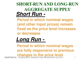
Long Run Aggregate Supply • In the long run, all costs and prices are variable • An increase in the price level will have no impact on Aggregate Supply in the long run because all firms' costs (e.g. wages and resource costs) will rise proportionally with the price level.

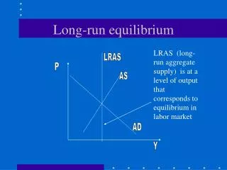
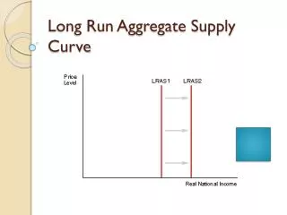
Long Run Aggregate Supply (cont) • In the long run, Aggregate Supply equals potential output • Prices adjust to costs, so the economy reaches efficiency • It is a level the economy tends toward • Thus, Long run Aggregate Supply (LAS) is vertical • It tells what economic output would be if nothing moves it from efficient resource use.

Long Run Aggregate Supply LAS Price level Real Output

Equilibrium: Short run and Long run • Short run equilibrium is where the economy is now. • It sets current output and the current price level • Long run equilibrium is where the economy is heading. • It always heads towards potential output (except for shocks that move it away) • LAS sets output, AD then sets long run prices

Long Run Equilibrium LAS Price level Long run equilibrium occurs when the SAS and AD intersect at LAS. Where the economy is, determined by the SAS and the AD, is where it is headed, determined by the LAS and AD. SAS Pe AD Ye Real Output

Disequilibrium • Disequilibrium occurs when the current output differs from potential output. • In a recessionary gap, current output is below potential output. Prices are above their long run equilibrium level. • In an inflationary gap, current output is above potential output. Prices are below their long run equilibrium level.

Disequilbrium: Recessionary Gap I LAS SAS Price level In a recessionary gap, actual output, Y2, is below potential output, Ye, which is given by the LAS. In this example, the recessionary price exceeds the equilibrium price. It was caused by a shift in the SAS P2 Pe AD Y2 Ye

Disequilbrium: Recessionary Gap I (cont) LAS SAS2 Price level We know in this case the recessionary gap was caused by a shift in the SAS because P2>Pe. SAS1 P2 Pe Y2 Ye

Disequilbrium: Recessionary Gap II LAS SAS Price level In a recessionary gap, actual output, Y2, is below potential output, Ye, which is given by the LAS. In the case shown, P2<Pe. Pe P2 AD Y2 Ye

Disequilbrium: Recessionary Gap II (cont) This recessionary gap was caused by a shift in the AD. LAS Price level SAS We know it was caused by a shift in AD because P2<Pe1. Notice, with the fall in AD, there is a new long run equilibrium price, Pe2. Pe1 P2 AD1 AD2 Y2 Ye

Review of Recessionary Gaps • When prices are above equilibrium level in a recessionary gap, the gap is caused by an upward shift in SAS • This means costs of production have increased, perhaps from increases in input prices. • When prices are below the equilibrium level in a recessionary gap, the gap is caused by a leftward shift in AD • This means something has lowered the demand for goods, like a decrease in exports.

Closing the Recessionary Gap • Recessionary gaps (like all gaps) if left alone, close as the SAS adjusts. • In a recessionary gap, there is are unused inputs. • Firms can pay inputs less, lowering the costs of production. • The gap closes as the SAS moves down.

Closing the Recessionary Gap In any recssionary gap with P1>Pe, the SAS shifts out from SAS1 to SAS2. Economic output grows, and prices fall. As any recessionary gap closes, economic output increases and prices fall. LAS SAS1 Price level SAS2 P1 Pe AD Y1 Ye

Disequilibrium: Inflationary Gaps • In an inflationary gap, current output exceeds long run equilibrium output, and current prices are below long run levels. • Inflationary gaps can also be caused by shifts in the AD or the SAS.

Inflationary Gaps I Here, the SAS has shifted out. Perhaps a new technology or newly discovered oil reserves lowered input prices, shifting the SAS out. Current output, Y2, exceeds potential output, Ye. The price level has fallen. LAS Price level SAS1 SAS2 Pe P2 AD Ye Y2

Inflationary Gaps II In this case, the AD has shifted out. Perhaps there was a tax cut, increased exports, or new government spending. Current output, Y2, exceeds potential output, Ye. The price level has increased. LAS Price level SAS1 P2 Pe AD2 AD1 Ye Y2

Closing the Inflationary Gap • Inflationary gaps (like recessionary gaps) if left alone, close as the SAS adjusts. • In a inflationary gap, there is a shortage of inputs. • To attract inputs firms pay more, raising the costs of production. • The gap closes as the SAS moves up.

Closing the Inflationary Gap In any inflationary gap P1<Pe. Shortages of inputs raise the cost of production, so the SAS shifts in from SAS1 to SAS2. Economic output falls, and prices go up. LAS Price level SAS2 SAS1 Pe P1 AD Ye Y1

Changes in Potential Output • Changes in potential output (LAS) can also cause gaps. • Questions: • What type of gap is created if there is real growth in the PPC? What are the long term outcomes for prices and output? • What type of gap is created if there is real loss in the PPC (it shifts inward)? What are the long term outcomes for prices and output?

Recessionary and Inflationary Gaps and Speed of Adjustment • In a recessionary gap, there is an excess supply of inputs, and there is pressure for wages and other inputs prices to fall. • Workers resist this drop in pay, so recessionary gaps close slowly. Output grows slowly as prices fall slowly. • In an inflationary gap, there is a shortage of inputs, and there is pressure for wages and other input prices to go up. • Workers are happy to get higher pay, so inflationary gaps close relatively fast. Output falls relatively quickly as prices rise.

Paradox of Thrift An increase in savings will shift the AD to the left (to AD’). This creates a recessionary gap, and output falls from Y1 to Yb. However, the increased savings means there is more investment possible, shifting the LAS out to LAS’, so the long term impact is higher NI and lower prices.

Policy Questions • The Japanese economy has been in doldrums for a long time. Japanese policy makers blame it on the high savings rate of the Japanese. Does this make sense? • Many analysts believe the US savings rate is too low. Many policies, for example, the Roth IRA, are designed to increase the savings rate. Discuss the short run and long run consequences of these policies.

Long Run Supply and Equilibrium