9.4 Perfect Competition Long Run Equilibrium

1. 9.4 Perfect Competition Long Run Equilibrium

2. Re-cap the Short Run • The short run is a timeframe in which at least one of the resource inputs used in production cannot be changed: • Positive/Negative Economic profits • or, Break-even • Break-even is what happens in the LONG RUN!

3. The Long Run • The short run is a timeframe in which at least one of the resource inputs used in production cannot be changed. • Exit and entry are long-run phenomena. • In the long run, all quantities of resources can be changed.

4. The Long Run • As long as D = P = MR > Min. SAVC pt. “b” • There is profits to be made (shaded area) • More firms (sellers) enter the market • Undercut the $9 price until reach $7 • More firms = more supply in SR, shifts to S1SR • Price lowers to $7 for ALL firms! • To compete firms have to lower production costs eg. pay lower wages • Move from SAC1 pt. “a” to SAC2 pt. “b”

5. Price Market S0SR S1SR $9 D1 D0 Quantity 0 1,200 840 Adjustments in LR Equilibrium Firm P S1 = MC1 SAC1 B LRATC1 SAC2 P1 = D = MR C a $7 b A 2.1 Q

6. An Increase in Demand • An increase in demand leads to higher prices and higher profits. pt “B” • Existing firms increase output. S0SR to S1SR • New firms enter the market, increasing output still more. • Price falls until all profit is competed away • pt “b”

7. Price Market S0SR S1SR $9 D1 D0 Quantity 0 1,200 840 Adjustments in LR Equilibrium Firm P S1 = MC1 SAC1 B LRATC1 SAC2 P1 = D = MR C a $7 b A 2.1 Q

8. An Increase in Demand • If input prices remain constant, the new equilibrium will be at the original price but with a higher output. pt. “C”

9. An Increase in Demand • The original firms return to their original output but since there are more firms in the market, the total market output increases where Q goes from: • 840 to 1,200

10. In the short run, the price does more of the adjusting. An Increase in Demand • In the long run, more of the adjustment is done by quantity.

11. The Predictions of the Model of Perfect Competition • A zero economic profit is a normal accounting profit, or just normal profit. • Firms produce where marginal cost equals price. • No one could be made better off without making someone else worse off. Economists refer to this result as economic efficiency.

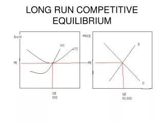
12. Long-Run Competitive Equilibrium • At long run equilibrium, economic profits are zero • The existence of losses will cause firms to leave the industry, market supply will decrease, and the price will increase until losses are zero Profits create incentives for new firms to enter, market supply will increase, and the price will fall until zero profits are made

13. Long-Run Competitive Equilibrium Graph P At long-run equilibrium, economic profits are zero MC LRATC SRATC P = D = MR Q

14. Long-Run Market Supply • In the long-run industry supply curve can take on 3 different shapes • Depending on input (eg wages, lettuce) costs increasing, decreasing or being constant

15. 9.5 Long-Run Industry Supply Curves • If the long-run industry supply curve is perfectly elastic, the market is a constant-cost industry • If the long-run industry supply curve is downward sloping, the market is a decreasing-cost industry If the long-run industry supply curve is upward sloping, the market is an increasing-cost industry

16. Long-Run Industry Supply Curves Constant-Cost Industries: • where the industry can increase output in the long-run without affecting input prices. Eg growing Cucumbers as a farmer, you can grow 100% more cucumbers this year but the cost of the seeds will remain the same

17. Long-Run Industry Supply Curves Constant-Cost Industries: • Demand for Cucumbers increase • price goes to P1 • Generate +ive economic profits, more firms enter the industry and current firms expand output to Qo • Supply shifts out to S1 • P goes back to Pe

18. Long-Run Industry Supply Curves Constant-Cost Industries

19. Long-Run Industry Supply Curves Constant-Cost Industries: Qe to Qo is the LRS

20. Long-Run Industry Supply Curves Increasing-Cost Industries: • where the industry increase output in the long-run which increases input prices. Eg coal mining gets more expensive as you produce more because the inputs used are so special and rare/unique

21. Long-Run Industry Supply Curves Increasing-Cost Industries: • Demand for Gold increase • price goes to P1 • Generate +ive economic profits, more firms enter the industry and current firms expand output to Qo • Cost of production rise so ATC and MC curves (= SR supply curves) rise • Supply shifts out to S1 • P goes to Po

22. Long-Run Industry Supply Curves Increasing-Cost Industries

23. Long-Run Industry Supply Curves Decreasing-Cost Industries: • where the industry increase output in the long-run which decreases input prices. Eg computer mftg. It gets less expensive as you produce more because technological advances used to make the inputs cause input prices to fall

24. Long-Run Industry Supply Curves Decreasing-Cost Industries: • Demand for Cucumbers increase • price goes to P1 • Generate +ive economic profits, more firms enter the industry and current firms expand output to Qo • Cost of production lower so ATC and MC curves (= SR supply curves) rise • Supply shifts out to S1 • P goes to Po

25. Long-Run Industry Supply Curves Decreasing-Cost Industries

26. 9.6 Social Evaluation of PC PC promotes • Productive Efficiency: Least Costly Combination of inputs Used in Production • Where, MR = MC at min LAVC and SAVC

27. Social Evaluation of PC PC promotes • Allocative Efficiency: a Combination of Resources Used in Production to Maximize Consumer Satisfaction • Where: • P, MR, MB (Demand) = MC (Supply) the price equals the opportunity costs to society of producing the last unit of that good ie marginal cost pricing eg.

28. Social Evaluation of PC PC promotes • Allocative Efficiency: a Combination of Resources Used in Production to Maximize Consumer Satisfaction

29. Normal Profit in the Long Run • Entry and exit occur whenever firms are earning more or less than “normal profit” (zero economic profit). • If firms are earning more than normal profit, other firms will have an incentive to enter the market. • If firms are earning less than normal profit, firms in the industry will have an incentive to exit the market.

30. Short Comings of PC Market Failure: Under/over allocating resources Negative Externality eg. Second hand smoking causes cancer in people who do not smoke. Smokers don’t have to pay any fine. If you don’t have to pay then you over allocate (over indulge)

31. Short Comings of PC Market Failure: Under/over allocating resources Positive Externality: Discovery of vaccine benefits us all. What we pay is little compared to how much it benefits us. From our point of view there can never be enough ie. it is underallocated.