Sample Size Determination for Health State Utility Comparisons
This poster explores consistency measures and sample size calculations in health state utility assessments across groups and time. It discusses differentiation score, inversion score, and more, along with methods to test validity.

Sample Size Determination for Health State Utility Comparisons
E N D
Presentation Transcript
Row 1 Row 2 Sample Size Determination in Studies Where Health State Utility Assessments Are Compared Across Groups & Time Barbara H Hanusa 1,2 Christopher R H Hanusa3, Chung-Chou (Joyce) H Chang2, & Kevin L Kraemer21. Department of Psychiatry, University of Pittsburgh, 2. Center for Research on Health Care, University of Pittsburgh, 3. Department of Mathematics, University of Washington • This Poster: • Describes the distributions of 3 consistency measures and the sample sizes needed to address the questions in the grant. • Measures of Consistency • Spearman’s ρ – Calculate ρ by 1 – 6T/[n2(n-1)], where T is the sum of the rank differences squared. This formula does not change when ties are allowed. • Differentiation Score & Inconsistency Index – Calculates the least number of rearrangements of health states necessary to achieve consistency, e.g. Inconsistency index of 143526 is two: 143526 – 124356 – 123456. Dividing by n-1 gives the index. This index takes on values between 0 and 1. When ties are allowed, calculate the number of rearrangements similarly but divide by n-nT, where nT is the maximum number of states tied. • Inversion Score – This measure calculates the number of adjacent inversions (or switches) required to achieve consistency. E.g.: Inversion score for 143526 is four: 143526 – 143256 – 134256 – 132456 – 123456. This measure takes on values between 0 and (n2-n)/2. When ties are included, calculate the number of inversions to find the non-decreasing ordering of the states, and if s states are tied, add (s2-s)/4 to your inversion score, e.g. Inversion score of 1 2 2 2 5.5 5.5 is 6/4+2/4=2 • First Set of Calculations • All possible permutations of 6 items are generated. • Ties were allowed in one of the rankings • Calculate the values of the 3 consistency measures for all • possible pairs (Figures in Column 1) • Second Set of Calculations • Set cutpoints on the values of the measure you want to consider evidence of validity. On the graphs in column 1 the vertical line indicates the most extreme 5% of the distributions. Use the values above the cutpoint to look at the distribution of the values in the restricted range. (Figures in Column 2) Two methods were considered to test whether an observed set of consistency values were compatible with the specified cutpoints. First, is to compare the observed distribution to the distributions of the type generated below – the distributions would have to be generated for the number of subjects in the study group and there would need to be iterations around the cutpoints of the distribution to maximize the power of the tests. Distributions could be compared with a series of Kolmogorov tests. Second, given the shapes of the distributions of the means of the rhos and the inversion measures and n per group > 10 you can use formulas for sample size developed for normally distributed data. Graphing the distributions with q-q plots showed that with n=20 the distributions differed only from normal at the tails of the distributions. At n=10, the Inconsistency Index distributions were not well distributed. The inversions and Spearman’s rho were. At n=20, the Inconsistency Index has larger standard deviations than the other measures. Column 1 Column 2 • Aims for the Parent Study • To develop and validate a method for assigning utility values to a spectrum of alcohol related health states in order to provide the information needed for a cost utility analysis of alcohol prevention and treatment programs (Grant submitted to NIAAA, Patient & Societal Utilities for Alcohol Problems, Kevin L. Kraemer, PI) • Statistical Issues • Estimate the study sample sizes required to demonstrate validity of utility values for a spectrum of alcohol related health states. Measures of validity are measures of consistency among multiple ratings at the individual subject level. Distributional information for two commonly used measures of consistency and one proposed measure need to be developed before the required sample sizes are estimated. • Background Information to Help Frame the Problem • Definitions • Cost Utility Analysis. Cost-Effectiveness Analysis (CEA) is used to compare the relative value of alternative programs for creating better health and/or longer life. Cost-Utility Analysis (CUA) is a special form of CEA where health-related quality of life is integrated into the effectiveness term. Before CUA can be completed values must be attached to different health states. • Alcohol Related Health States (ARHS) –These describe different points on the continuum of alcohol use and problems, ranging from non-drinking to alcohol dependence with life threatening alcohol related diseases and alcohol dependent patients in treatment and recovery. Theoretically there are 11 medically plausible and differentiable health states. Subjects will rate 6. • What do subjects do? What are the dependent measures? • Definitions • Ranking – Subjects are presented with descriptions of 11 alcohol related health states and a control condition (for this study, blindness). They are asked to rank these states in terms of their preference. As a second control state, they are asked to include their own state of health in the ranking. • Rating – Using a laptop computer subjects rate the health states with three different methods. To reduce subject burden the subjects will only rate 6 health states but must rate them with all methods. • Visual Analog Scale (VAS) subjects use a vertical scale with Perfect Health (utility=1) on the top and death (utility = 0) at the bottom. Subjects are asked to rate the described health state on the scale. • Time Trade Off (TTO) Subjects are asked to imagine they had to live 20 years in the described health state. Subjects who are willing to trade away some time in the health state to live in perfect health but who also prefer the health state to death have a utility rating greater than 0.0 and less than 1.0. • Standard Gamble (SG) Subjects are again shown the health states and asked whether he/she would accept a 0% risk of death for a treatment with a 100% chance of curing the health state and restoring perfect health. Subjects who are willing to accept some risk of death less than 100% have a utility rating greater than 0.0 and less than 1.0 for the health state. For example, a subject who is willing to accept a maximal risk of death of 2% to have a 98% chanceof cure and perfect health has a utility for the health state of 0.98 (1 – 0.02). • Gold Standard. For testing the validity of the rankings and the ratings the ARHS are constructed in such a way that from the medical perspective there is a ‘rational judge’ way to rank (but not assign numerical values) the ARHSs. • Conclusions • Both Spearman’s Rho and Inversion Score give normal distributions when 10-member samples are taken; whereas Inconsistency Index does not. By n=20, the distribution of mean Inconsistency Index has a ‘normal’ distribution. The standard deviations of the samples of means for rho and IVs are smaller and consequently lead to smaller required sample sizes. • Although not the initial focus of the analyses it became clear that the IC index is a poor choice for a measure of consistency when there are few states rated – this is usually the case – implying that other measures should be used. • The Inversion Score measure represents what logical processes subjects use to change their opinions, so it is a better suited metric than Spearman’s rho is. The Inversion Score Distribution is within a small error of normal when n ≥7. (Hofri, 1987) Third Set of Calculations Using different cutpoints for the restricted ranges of the measures generate 2000 random samples of size 10 & 20 from the restricted range and calculate the mean values of the measure for each sample. Plot the distribution of means. Figures in Row 1 are the distributions with n=10, in Row 2 the distributions with n=20.

