Download
1 / 30
300 likes | 358 Vues
Learn about the types of measures used to analyze variation and how to calculate range, variance, and standard deviation. Apply the Empirical Rule and Chebychev's Theorem in specific situations.

E N D
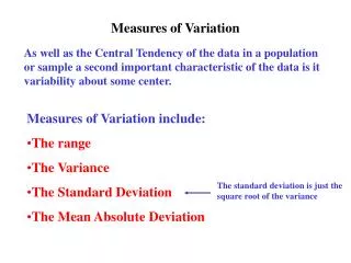
Descriptive StatisticsMeasures of Variation Essentials Measures of Variation Range Variance Standard Deviation Interquartile Range (in Measures of Position) Empirical Rule Chebychev’s Theorem (in Additional Topics) Example Additional Topics
Essentials:Measures of Variation(Variation – a must for statistical analysis.) • Know the types of measures used to look at variation and the type data to which they apply. • Be able to calculate the range, standard deviation and inter-quartile range. • Be able to determine the distance away from the mean a given value lies in terms of standard deviations (think z-score). • Be able to apply the Empirical Rule and Chebychev’s Theorem to specific situations.
Measures of Variation Range Variance Standard Deviation Interquartile Range (IQR; see Measures of Position)
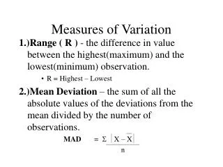
Range The Range of a data set is the difference between the highest value and the lowest value. Example: Given the following data values, identify the range of the distribution. Values: 2, 4, 6, 8, 10 Range = 10 – 2 = 8
Variance For a sample the variance is a measure of variation equal to the sum of the squared deviation scores divided by n-1. It is also the square of the standard deviation. Sample Variance:
Sample Standard Deviation Standard deviation is a measure of the typical amount an entry deviates (or varies) from the mean. The more the entries are spread out, the greater the standard deviation. Sample Standard Deviation(s): Definition Formula Calculation Formula
Interpreting Standard Deviation Larson/Farber 4th ed. Standard deviation is a measure of the typical amount an entry deviates from the mean. The more the entries are spread out, the greater the standard deviation.
Anatomy of the Standard Deviation The Standard Deviation is the most used measure of dispersion (how spread out the data are from one another). The value of the Standard Deviation tells us how closely the values of observations for a data set are clustered around the mean. A lower value of the Standard Deviation for a data set indicates that the values of that data set are spread over a relatively smaller range around the mean. A large value of the Standard Deviation for a data set indicates that the values of that data set are spread over a relatively larger range around the mean. NOTATION When we refer to the Population Standard Deviation, it is denoted by When we refer to the Sample Standard Deviation, it is denoted by s
Interpreting Standard Deviation: Empirical Rule (68 – 95 – 99.7 Rule) • About 68.26%of the data lie within one standard deviation of the mean. • About95.44%of the data lie within two standard deviations of the mean. • About99.74%of the data lie within three standard deviations of the mean. For data with a (symmetric) bell-shaped distribution, the standard deviation has the following characteristics:
Interpreting Standard Deviation: Empirical Rule (68 – 95 – 99.7 Rule) 99.7% within 3 standard deviations 95% within 2 standard deviations 68% within 1 standard deviation 34% 34% 2.35% 2.35% 13.5% 13.5% Source: Larson/Farber 4th ed.
Example: Using the Empirical Rule Source: Larson/Farber 4th ed. Example: In a survey conducted by the National Center for Health Statistics, the sample mean height of women in the United States (ages 20-29) was 64 inches, with a sample standard deviation of 2.71 inches. Estimate the percent of the women whose heights are between 64 inches and 69.42 inches.
Solution: Using the Empirical Rule • Because the distribution is bell-shaped, you can use the Empirical Rule. 34% 13.5% 55.87 58.58 61.29 64 66.71 69.42 72.13 34% + 13.5% = 47.5% of women are between 64 and 69.42 inches tall. (64 + 2.71 = 66.71 + 2.71 = 69.42; all inches) Source: Larson/Farber 4th ed.
Range Rule of Thumb To obtain a rough estimate of the standard deviation, s, Conversely, the “minimum” value would be approximately equal to the mean – 2*(standard deviation). The “maximum” value would be approximately equal to the mean + 2*(standard deviation).
Population Variance & Standard Deviation The population variance, s2 (sigma-squared) is a measure of variation equal to the sum of the squared deviation scores divided by N. It is also the square of the standard deviation. Population Variance: Population Standard Deviation:
Chebyshev’s Theorem The Empirical Rule applies if the distribution of the data is approximately bell-shaped. Chebyshev’s Theorem applies to distributions regardless of shape. It states that the proportion (fraction) of data lying within K standard deviations of the mean is always at least 1 – 1/K2, where K is any possible number > 1. When K = 2: At least 3/4 (75%) of all values lie within 2 standard deviations of the mean. When K = 3: At least 8/9 (89%) of all values lie within 3 standard deviations of the mean.
Example: Using Chebychev’s Theorem Source: Larson/Farber 4th ed. The age distribution for Florida is shown in the histogram. Apply Chebychev’s Theorem to the data using k = 2. What can you conclude?
Solution: Using Chebychev’s Theorem At least 75% of the population of Florida is between 0 and 88.8 years old. Given k = 2: • Two S.D. below the mean = μ – 2σ = 39.2 – 2(24.8) = -10.4 (use 0 since age can’t be negative) • Two S.D. above the mean = μ + 2σ = 39.2 + 2(24.8) = 88.8 Source: Larson/Farber 4th ed.
Empirical Rule (68-95-99.7 Rule) The Empirical Rule states that if the distribution of the data is approximately bell-shaped, then: Approx. 68.26% of the observations fall within 1 standard deviation of the mean. Approx. 95.44% of the observations fall within 2 standard deviations of the mean. Approx. 99.74% of the observations fall within 3 standard deviations of the mean.
Empirical Rule 99.7% of data are within 3 standard deviations of the mean 95% within 2 standard deviations 68% within 1 standard deviation 34% 34% 2.4% 2.4% 0.1% 0.1% 13.5% 13.5% x - 3s x - 2s x - s x x+s x+2s x+3s
Chebychev’s Theorem • k = 2: In any data set, at least of the data lie within 2 standard deviations of the mean. • k = 3: In any data set, at least of the data lie within 3 standard deviations of the mean. Source: Larson/Farber 4th ed. The portion of any data set lying within k standard deviations (k > 1) of the mean is at least:
Example: Using Chebychev’s Theorem The age distribution for Florida is shown in the histogram. Apply Chebychev’s Theorem to the data using k = 2. What can you conclude? Larson/Farber 4th ed. 23
Solution: Using Chebychev’s Theorem At least 75% of the population of Florida is between 0 and 88.8 years old. Source: Larson/Farber 4th ed. Given k = 2: μ – 2σ = 39.2 – 2(24.8) = -10.4 (use 0 since age can’t be negative) μ + 2σ = 39.2 + 2(24.8) = 88.8
Interquartile Range (IQR) The Interquartile Range is a measure of variation. It is the difference between the first quartile, Q1(25th percentile) and the third quartile, Q3 (75th percentile).
The Interquartile Range enables us to determine the existence of outliers. Outliers exist in a data set if any of the values are Less than or Greater than
Outliers An Outlier is a value (or values) that is located very far away from almost all of the other values in a data set. An outlier can: Have a dramatic effect on the mean. Have a dramatic effect on the standard deviation. Have an effect so dramatic on the scale of a histogram that the true nature of the distribution is totally obscured.
Finding a Standard Deviation From a Frequency Table To find a standard deviation when data is presented in the form of a frequency table As was the case when the mean from a frequency table, was calculated, x is the class midpoint.
Standard Deviation Standard Deviation – a measure of variation of values about the mean. Sample Standard Deviation Population Standard Deviation
A) “Loui’villeB) “Lewis”ville What is the correct pronunciation of the capital of Kentucky?