Analyzing Input Purchasing: Monopsony, Monopoly, and Perfect Competition Cases
This analysis explores four distinct cases of input purchasing, dissecting the equilibrium conditions in various market structures—monopsonist and monopolist interactions, perfect competition in input purchasing, and the interplay of monopolistic sellers with perfectly competitive input suppliers. Each case illustrates the principles of Marginal Revenue Product (MRP) and Marginal Input Cost (MIC), highlighting how these factors determine the quantity and price of inputs purchased. Insights shed light on market dynamics affecting input pricing.

Analyzing Input Purchasing: Monopsony, Monopoly, and Perfect Competition Cases
E N D
Presentation Transcript
1 Page 161
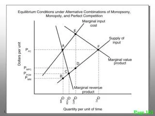
Case #1: Monopsonist in input purchasing and Monopolist seller of product • Equilibrium: MRP=MIC at Pt A • Pricing off input supply curve gives QMM and PMM at B MIC Supply of Input A $ per unit of input Note: Use MR not output price (PY) due to being a monopolist (I don’t display the MVP curve) PMM B MRP=MR x MPP QMM Amount of Input Purchased 2 Page 161
Case #2: Perfect Competition in input purchasing andMonopoly seller • Equilibrium is where MRP=Input price, PPCM • No Marginal Input Cost curve → QPCM and PPCM Input price determined by input market (take input price as given $ per unit of input PPCM MRP=MR x MPP QMM 3 Amount of Input Purchased Page 161
Case #3: Monopsony in input purchasing and Perfectly Competitive seller • Equilibrium: MVP=MIC at Pt. E • Pricing off supply curve → QMPC and PMPC at Pt. D MIC E Supply of Input $ per unit of input PMPC D MVP=PY x MPP We use MVP instead of MRP curve given P.C. seller QMPC 4 Amount of Input Purchased Page 161
Case #4: Perfect Competition in both input purchasing and product sales • Equilibrium: MVP=Input Price at Pt. F • → QPC and PPC MVP=PY x MPP Input price determined by input market $ per unit of input PPC QPC 5 Amount of Input Purchased Page 161