Download
1 / 1
10 likes | 138 Vues
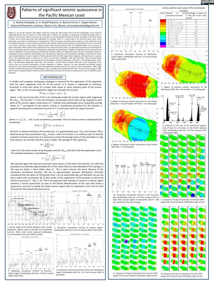
Colors code for each value of the convolution function. Patterns of significant seismic quiescence in the Pacific Mexican coast. A. Muñoz- Diosdado , A. H. Rudolf-Navarro, A. Barrera-Ferrer, F. Angulo-Brown National Polytechnic Institute, Mexico City, Mexico, amunozdiosdado@gmail.com .

E N D
Colors code for each value of the convolution function Patterns of significant seismic quiescence in the Pacific Mexican coast A. Muñoz-Diosdado, A. H. Rudolf-Navarro, A. Barrera-Ferrer, F. Angulo-Brown National Polytechnic Institute, Mexico City, Mexico, amunozdiosdado@gmail.com Mexico is one of the countries with higher seismicity. During the 20th century, 8% of all the earthquakes in the world of magnitude greater than or equal to 7.0 have taken place in Mexico. On average, an earthquake of magnitude greater than or equal to 7.0 occurred in Mexico every two and a half years. Great earthquakes in Mexico have their epicenters in the Pacific Coast in which some seismic gaps have been identified; for example, there is a mature gap in the Guerrero State Coast, which potentially can produce an earthquake of magnitude 8.2. With the purpose of making some prognosis, some researchers study the statistical behavior of certain physical parameters that could be related with the process of accumulation of stress in the Earth crust. Other researchers study seismic catalogs trying to find seismicity patterns that are manifested before the occurrence of great earthquakes. Many authors have proposed that the study of seismicity rates is an appropriate technique for evaluating how close a seismic gap may be to rupture. We designed an algorithm for identification of patterns of significant seismic quiescence by using the definition of seismic quiescence proposed by Schreider (1990). This algorithm shows the area of quiescence where an earthquake of great magnitude will probably occur. We apply our algorithm to the earthquake catalogue of the Mexican Pacific coast located between 14 and 21 degrees of North latitude and 94 and 106 degrees West longitude; with depths less or equal to 60 km and magnitude greater or equal to 4.2, which occurred from September, 1965 until December, 2014. We have found significant patterns of seismic quietude before the earthquakes of Oaxaca (November1978, Mw = 7.8), Petatlán (March 1979, Mw = 7.6), Michoacán (September 1985, Mw = 8.0, and Mw = 7.6) and Colima (October 1995, Mw = 8.0). Fortunately, in this century have not occurred earthquakes of great magnitude in Mexico, however, we have identified well-defined seismic quiescence in the Guerrero seismic-gap, which are apparently correlated with the occurrence of silent earthquakes in 2002, 2006 and 2011 recently discovered by GPS technology. In fact, a possible silent earthquake with Mw =7.6 occurred at this gap in 2002 which lasted for approximately 4 months and was detected by continuous GPS receivers located over an area of 550x250 squarekilometers. 5. Temporary convolution function of Michoacán-Colima region. Earthquakes with MS ≥ 4.3 from January 1965 to April 2012 METHODOLOGY A reliable and complete earthquake catalogue is required for the application of the algorithm with the same magnitude scale for all the events. It is chosen a magnitude as minimum threshold. A circle with radius R is chosen with center in some arbitrary point of the seismic region. Then, in the circular exploration region we calculate the function 7. Region of previous seismic quiescence to the Michoacán 1985, Mw = 8.0 and Mw = 7.6 earthquakes where is the occurrence time of the n-th earthquake inside the circular region, with magnitude M ≥ Mmin. The function T’ is the time between consecutive events that can be assigned to each point of the seismic region; small values of T’ indicate that earthquakes occur frequently, and big values of T’ correspond to low seismic activity. A smoothness procedure for the function is applied calculating the convolution function of T’ in each point with the Laplace function 6. Region of previous seismic quiescence to the Oaxaca 1978, Mw = 7.8 and Petatlán 1979 Mw = 7.6 earthquakes where n = 1, 2, 3, ... and s is the smoothness parameter. The k-th seismic event is related with the convolution 9. Evolution of the size of the quiescence regions, area of level 2σ and major, in the Pacific Mexican coast. Earthquakes with MS ≥ 4.6 from January 1975 to December 2002 the limit l is determined when the function f(n, s) is approximately zero. Thus, the function T(k) is determined by three parameters: Mmin, R and s, which are chosen in an arbitrary way. To identify a period of seismic quiescence it is necessary to know the average value of T(k) calculated in a big time interval, we consider that this value is stable. The average of T(k) is given by 8. Region of previous seismic quiescence to the Colima 1995, Mw = 7.9 earthquake where N is the total number of earthquakes with M ≥ Mmin that fall inside the exploration circle. The standard deviation is calculated as We calculate again the value but now with those values of T(k) within the interval ± 2σ; with this procedure we eliminate approximately 5% of the values that are more deviated of the average, in this way we obtain a more stable value of . The σ value remains the same. Because of the temporary convolution function T(k) has an approximately Gaussian distribution, Schreider considered that the values of T(k) greater than ± 3σ are abnormally big, and therefore we can say that a point with coordinates (φ, λ) (the center of the exploration circle) presents an abnormal seismic quiescence if T(k) ≥ ± 3σ. This is the approach that indicates if a point in a seismic region presents a seismic quiescence; to pass to the formal determination of the area that shows a quiescence, we have to sweepthe whole seismic region with an exploration circle and to mark those points that present the quiescence. 10. Temporary convolution function in the Guerrero-gap. Earthquakes with MS ≥ 4.3 from January 1975 to April 2012; circular region of exploration with R = 250 Km, centered in the Guerrero gap 11. Sequence of maps of seismicity since March 1994 (upper left corner) to March 1996 (lower right corner). 1. Seismic region of the Pacific Mexican coast, circular exploration regions used to calculate the convolution function. Other small circles represent earthquakes occurred between the years 1965 and 2001 2. Temporary convolution function of Oaxaca region. Earthquakes with MS ≥ 4.3 from January 1965 to April 2012 4. Temporary convolution function of Guerrero-Michoacán region. Earthquakes with MS ≥ 4.3 from January 1965 to April 2012 3. Temporary convolution function of Guerrero - Oaxaca region. Earthquakes with MS ≥ 4.3 from January 1965 to April 2012. 12. Sequence of maps of seismicity since January 2013 (upper left corner) to March 2014 (lower right corner). 13. Sequence of maps of seismicity since June 1976 (upper left corner) to July 1978 (lower right corner).