Download
1 / 60
600 likes | 785 Vues
EE898.02 Architecture of Digital Systems Lecture 1 Review of Pipelines, Performance, Caches, and Virtual Memory(!). September 17, 2004 Prof. Seok-Bum Ko Electrical Engineering University of Saskatchewan. A. B. C. D. Pipelining: Its Natural!. Laundry Example

E N D
EE898.02Architecture of Digital SystemsLecture 1 Review of Pipelines, Performance, Caches, and Virtual Memory(!) September 17, 2004 Prof. Seok-Bum Ko Electrical Engineering University of Saskatchewan
A B C D Pipelining: Its Natural! • Laundry Example • Ann, Brian, Cathy, Dave each have one load of clothes to wash, dry, and fold • “Washer” takes 30 minutes • “Dryer” takes 40 minutes • “Folder” takes 20 minutes
A B C D Sequential Laundry 6 PM Midnight 7 8 9 11 10 Time • Sequential laundry takes 6 hours for 4 loads • If they learned pipelining, how long would laundry take? 30 40 20 30 40 20 30 40 20 30 40 20 T a s k O r d e r
30 40 40 40 40 20 A B C D Pipelined LaundryStart work ASAP 6 PM Midnight 7 8 9 11 10 • Pipelined laundry takes 3.5 hours for 4 loads Time T a s k O r d e r
30 40 40 40 40 20 A B C D Pipelining Lessons 6 PM 7 8 9 Time • Pipelining doesn’t help latency of single task, it helps throughput of entire workload • Pipeline rate limited by slowest pipeline stage • Multiple tasks operating simultaneously • Potential speedup = Number pipe stages • Unbalanced lengths of pipe stages reduces speedup • Time to “fill” pipeline and time to “drain” it reduces speedup T a s k O r d e r
Computer Pipelines • Execute billions of instructions, so throughput is what matters • What is desirable in instruction sets for pipelining? • Variable length instructions vs. all instructions same length? • Memory operands part of any operation vs. memory operands only in loads or stores? • Register operand many places in instruction format vs. registers located in same place?
A "Typical" RISC • 32-bit fixed format instruction (3 formats) • Memory access only via load/store instructions • 32 32-bit GPR (R0 contains zero, DP take pair) • 3-address, reg-reg arithmetic instruction; registers in same place • Single address mode for load/store: base + displacement • no indirection • Simple branch conditions • Delayed branch see: SPARC, MIPS, HP PA-Risc, DEC Alpha, IBM PowerPC, CDC 6600, CDC 7600, Cray-1, Cray-2, Cray-3
Example: MIPS (Note register location) Register-Register 6 5 11 10 31 26 25 21 20 16 15 0 Op Rs1 Rs2 Rd Opx Register-Immediate 31 26 25 21 20 16 15 0 immediate Op Rs1 Rd Branch 31 26 25 21 20 16 15 0 immediate Op Rs1 Rs2/Opx Jump / Call 31 26 25 0 target Op
Adder 4 Address Inst ALU 5 Steps of MIPS DatapathFigure A.17, Page A-29, CA:AQA 3e Instruction Fetch Instr. Decode Reg. Fetch Execute Addr. Calc Memory Access Write Back Next PC MUX Next SEQ PC Zero? RS1 Reg File MUX RS2 Memory Data Memory L M D RD MUX MUX Sign Extend Imm WB Data
MEM/WB ID/EX EX/MEM IF/ID Adder 4 Address ALU 5 Steps of MIPS DatapathFigure A.18, Page A-31 , CA:AQA 3e Instruction Fetch Execute Addr. Calc Memory Access Instr. Decode Reg. Fetch Write Back Next PC MUX Next SEQ PC Next SEQ PC Zero? RS1 Reg File MUX Memory RS2 Data Memory MUX MUX Sign Extend WB Data Imm RD RD RD • Data stationary control • local decode for each instruction phase / pipeline stage
Reg Reg Reg Reg Reg Reg Reg Reg Ifetch Ifetch Ifetch Ifetch DMem DMem DMem DMem ALU ALU ALU ALU Cycle 1 Cycle 2 Cycle 3 Cycle 4 Cycle 5 Cycle 6 Cycle 7 Visualizing PipeliningFigure 3.3, Page 133 , CA:AQA 2e Time (clock cycles) I n s t r. O r d e r
It’s Not That Easy for Computers • Limits to pipelining: Hazards prevent next instruction from executing during its designated clock cycle • Structural hazards: HW cannot support this combination of instructions (single person to fold and put clothes away) • Data hazards: Instruction depends on result of prior instruction still in the pipeline (missing sock) • Control hazards: Caused by delay between the fetching of instructions and decisions about changes in control flow (branches and jumps).
Reg Reg Reg Reg Reg Reg Reg Reg Reg Reg Ifetch Ifetch Ifetch Ifetch DMem DMem DMem DMem ALU ALU ALU ALU ALU One Memory Port/Structural HazardsFigure A.4, Page A-14 Time (clock cycles) Cycle 1 Cycle 2 Cycle 3 Cycle 4 Cycle 5 Cycle 6 Cycle 7 I n s t r. O r d e r Load DMem Instr 1 Instr 2 Instr 3 Ifetch Instr 4
Reg Reg Reg Reg Reg Reg Reg Reg Ifetch Ifetch Ifetch Ifetch DMem DMem DMem ALU ALU ALU ALU Bubble Bubble Bubble Bubble Bubble One Memory Port/Structural HazardsFigure A.5, Page A-15, CA:AQA 3e Time (clock cycles) Cycle 1 Cycle 2 Cycle 3 Cycle 4 Cycle 5 Cycle 6 Cycle 7 I n s t r. O r d e r Load DMem Instr 1 Instr 2 Stall Instr 3
Reg Reg Reg Reg Reg Reg Reg Reg Reg Reg ALU ALU ALU ALU ALU Ifetch Ifetch Ifetch Ifetch Ifetch DMem DMem DMem DMem DMem EX WB MEM IF ID/RF I n s t r. O r d e r add r1,r2,r3 sub r4,r1,r3 and r6,r1,r7 or r8,r1,r9 xor r10,r1,r11 Data Hazard on R1Figure A.6, page A-17 Time (clock cycles)
Three Generic Data Hazards • Read After Write (RAW)InstrJ tries to read operand before InstrI writes it • Caused by a “Dependence” (in compiler nomenclature). This hazard results from an actual need for communication. I: add r1,r2,r3 J: sub r4,r1,r3
I: sub r4,r1,r3 J: add r1,r2,r3 K: mul r6,r1,r7 Three Generic Data Hazards • Write After Read (WAR)InstrJ writes operand before InstrI reads it • Called an “anti-dependence” by compiler writers.This results from reuse of the name “r1”. • Can’t happen in MIPS 5 stage pipeline because: • All instructions take 5 stages, and • Reads are always in stage 2, and • Writes are always in stage 5
I: sub r1,r4,r3 J: add r1,r2,r3 K: mul r6,r1,r7 Three Generic Data Hazards • Write After Write (WAW)InstrJ writes operand before InstrI writes it. • Called an “output dependence” by compiler writersThis also results from the reuse of name “r1”. • Can’t happen in MIPS 5 stage pipeline because: • All instructions take 5 stages, and • Writes are always in stage 5 • Will see WAR and WAW in later more complicated pipes
Reg Reg Reg Reg Reg Reg Reg Reg Reg Reg ALU ALU ALU ALU ALU Ifetch Ifetch Ifetch Ifetch Ifetch DMem DMem DMem DMem DMem Forwarding to Avoid Data HazardFigure A. 7, Page A-18 Time (clock cycles) I n s t r O r d e r add r1,r2,r3 sub r4,r1,r3 and r6,r1,r7 or r8,r1,r9 xor r10,r1,r11
ALU HW Change for ForwardingFigure A. 23, Page A-37 ID/EX EX/MEM MEM/WR NextPC mux Registers Data Memory mux mux Immediate
Reg Reg Reg Reg Reg Reg Reg Reg ALU Ifetch Ifetch Ifetch Ifetch DMem DMem DMem DMem ALU ALU ALU ldr1, 0(r2) I n s t r. O r d e r dsub r4,r1,r6 and r6,r1,r7 or r8,r1,r9 Data Hazard Even with ForwardingFigure A. 9, Page A-20 Time (clock cycles)
Reg Reg Reg Ifetch Ifetch Ifetch Ifetch DMem ALU Bubble ALU ALU Reg Reg DMem DMem Bubble Reg Reg Data Hazard Even with ForwardingFigure A.10, Page A-21 , CA:AQA 3e Time (clock cycles) I n s t r. O r d e r ldr1, 0(r2) sub r4,r1,r6 and r6,r1,r7 Bubble ALU DMem or r8,r1,r9
Software Scheduling to Avoid Load Hazards Try producing fast code for a = b + c; d = e – f; assuming a, b, c, d ,e, and f in memory. Slow code: LW Rb,b LW Rc,c ADD Ra,Rb,Rc SW a,Ra LW Re,e LW Rf,f SUB Rd,Re,Rf SW d,Rd Fast code: LW Rb,b LW Rc,c LW Re,e ADD Ra,Rb,Rc LW Rf,f SW a,Ra SUB Rd,Re,Rf SW d,Rd
Reg Reg Reg Reg Reg Reg Reg Reg Reg Reg ALU ALU ALU ALU ALU Ifetch Ifetch Ifetch Ifetch Ifetch DMem DMem DMem DMem DMem 10: beq r1,r3,36 14: and r2,r3,r5 18: or r6,r1,r7 22: add r8,r1,r9 36: xor r10,r1,r11 Control Hazard on BranchesThree Stage Stall
Example: Branch Stall Impact • If 30% branch, Stall 3 cycles significant • Two part solution: • Determine branch taken or not sooner, AND • Compute taken branch address earlier • MIPS branch tests if register = 0 or 0 • MIPS Solution: • Move Zero test to ID/RF stage • Adder to calculate new PC in ID/RF stage • 1 clock cycle penalty for branch versus 3
MEM/WB ID/EX EX/MEM IF/ID Adder 4 Address ALU Pipelined MIPS DatapathFigure 3.22, page 163, CA:AQA 2/e Instruction Fetch Execute Addr. Calc Memory Access Instr. Decode Reg. Fetch Write Back Next SEQ PC Next PC MUX Adder Zero? RS1 Reg File Memory RS2 Data Memory MUX MUX Sign Extend WB Data Imm RD RD RD • Data stationary control • local decode for each instruction phase / pipeline stage
Four Branch Hazard Alternatives #1: Stall until branch direction is clear #2: Predict Branch Not Taken • Execute successor instructions in sequence • “Squash” instructions in pipeline if branch actually taken • Advantage of late pipeline state update • 47% MIPS branches not taken on average • PC+4 already calculated, so use it to get next instruction #3: Predict Branch Taken • 53% MIPS branches taken on average • But haven’t calculated branch target address in MIPS • MIPS still incurs 1 cycle branch penalty • Other machines: branch target known before outcome
Four Branch Hazard Alternatives #4: Delayed Branch • Define branch to take place AFTER a following instruction branch instruction sequential successor1 sequential successor2 ........ sequential successorn branch target if taken • 1 slot delay allows proper decision and branch target address in 5 stage pipeline • MIPS uses this Branch delay of length n
Delayed Branch • Where to get instructions to fill branch delay slot? • Before branch instruction • From the target address: only valuable when branch taken • From fall through: only valuable when branch not taken • Canceling branches allow more slots to be filled • Compiler effectiveness for single branch delay slot: • Fills about 60% of branch delay slots • About 80% of instructions executed in branch delay slots useful in computation • About 50% (60% x 80%) of slots usefully filled • Delayed Branch downside: 7-8 stage pipelines, multiple instructions issued per clock (superscalar)
DC to Paris Speed Passengers Throughput (pmph) 6.5 hours 610 mph 470 286,700 3 hours 1350 mph 132 178,200 Which is faster? Plane Boeing 747 BAD/Sud Concodre • Time to run the task (ExTime) • Execution time, response time, latency • Tasks per day, hour, week, sec, ns … (Performance) • Throughput, bandwidth
performance(x) = 1 execution_time(x) Performance(X) Execution_time(Y) n = = Performance(Y) Execution_time(x) Definitions • Performance is in units of things per sec • bigger is better • If we are primarily concerned with response time " X is n times faster than Y" means
CPU time = Seconds = Instructions x Cycles x Seconds Program Program Instruction Cycle Aspects of CPU Performance (CPU Law) Inst Count CPI Clock Rate Program X Compiler X (X) Inst. Set. X X Organization X X Technology X
Cycles Per Instruction(Throughput) “Average Cycles per Instruction” • CPI = (CPU Time * Clock Rate) / Instruction Count • = Cycles / Instruction Count “Instruction Frequency”
Example: Calculating CPI Base Machine (Reg / Reg) Op Freq Cycles CPI(i) (% Time) ALU 50% 1 .5 (33%) Load 20% 2 .4 (27%) Store 10% 2 .2 (13%) Branch 20% 2 .4 (27%) 1.5 Typical Mix of instruction types in program
Example: Branch Stall Impact • Assume CPI = 1.0 ignoring branches • Assume solution was stalling for 3 cycles • If 30% branch, Stall 3 cycles • Op Freq Cycles CPI(i) (% Time) • Other 70% 1 .7 (37%) • Branch 30% 4 1.2 (63%) • => new CPI = 1.9, or almost 2 times slower
Example 2: Speed Up Equation for Pipelining For simple RISC pipeline, CPI = 1:
Example 3: Evaluating Branch Alternatives (for 1 program) Scheduling Branch CPI speedup v. scheme penalty stall Stall pipeline 3 1.42 1.0 Predict taken 1 1.14 1.26 Predict not taken 1 1.09 1.29 Delayed branch 0.5 1.07 1.31 Conditional & Unconditional = 14%, 65% change PC
Example 4: Dual-port vs. Single-port • Machine A: Dual ported memory (“Harvard Architecture”) • Machine B: Single ported memory, but its pipelined implementation has a 1.05 times faster clock rate • Ideal CPI = 1 for both • Loads are 40% of instructions executed SpeedUpA = Pipeline Depth/(1 + 0) x (clockunpipe/clockpipe) = Pipeline Depth SpeedUpB = Pipeline Depth/(1 + 0.4 x 1) x (clockunpipe/(clockunpipe / 1.05) = (Pipeline Depth/1.4) x 1.05 = 0.75 x Pipeline Depth SpeedUpA / SpeedUpB = Pipeline Depth/(0.75 x Pipeline Depth) = 1.33 • Machine A is 1.33 times faster
Recap: Who Cares About the Memory Hierarchy? Processor-DRAM Memory Gap (latency) µProc 60%/yr. (2X/1.5yr) 1000 CPU “Moore’s Law” 100 Processor-Memory Performance Gap:(grows 50% / year) Performance 10 DRAM 9%/yr. (2X/10 yrs) DRAM 1 1980 1981 1982 1983 1984 1985 1986 1987 1988 1989 1990 1991 1992 1993 1994 1995 1996 1997 1998 1999 2000 Time
Levels of the Memory Hierarchy Upper Level Capacity Access Time Cost Staging Xfer Unit faster CPU Registers 100s Bytes <1s ns Registers prog./compiler 1-8 bytes Instr. Operands Cache 10s-100s K Bytes 1-10 ns $10/ MByte Cache cache cntl 8-128 bytes Blocks Main Memory M Bytes 100ns- 300ns $1/ MByte Memory OS 512-4K bytes Pages Disk 10s G Bytes, 10 ms (10,000,000 ns) $0.0031/ MByte Disk user/operator Mbytes Files Larger Tape infinite sec-min $0.0014/ MByte Tape Lower Level
The Principle of Locality • The Principle of Locality: • Program access a relatively small portion of the address space at any instant of time. • Two Different Types of Locality: • Temporal Locality (Locality in Time): If an item is referenced, it will tend to be referenced again soon (e.g., loops, reuse) • Spatial Locality (Locality in Space): If an item is referenced, items whose addresses are close by tend to be referenced soon (e.g., straightline code, array access) • Last 15 years, HW (hardware) relied on locality for speed
Lower Level Memory Upper Level Memory To Processor Blk X From Processor Blk Y Memory Hierarchy: Terminology • Hit: data appears in some block in the upper level (example: Block X) • Hit Rate: the fraction of memory access found in the upper level • Hit Time: Time to access the upper level which consists of RAM access time + Time to determine hit/miss • Miss: data needs to be retrieve from a block in the lower level (Block Y) • Miss Rate = 1 - (Hit Rate) • Miss Penalty: Time to replace a block in the upper level + Time to deliver the block the processor • Hit Time << Miss Penalty (500 instructions on 21264!)
Cache Measures • Hit rate: fraction found in that level • So high that usually talk about Miss rate • Miss rate fallacy: as MIPS to CPU performance, miss rate to average memory access time in memory • Average memory-access time = Hit time + Miss rate x Miss penalty (ns or clocks) • Miss penalty: time to replace a block from lower level, including time to replace in CPU • access time: time to lower level = f(latency to lower level) • transfer time: time to transfer block =f(BW between upper & lower levels)
Simplest Cache: Direct Mapped Memory Address Memory 0 4 Byte Direct Mapped Cache 1 Cache Index 2 • Location 0 can be occupied by data from: • Memory location 0, 4, 8, ... etc. • In general: any memory locationwhose 2 LSBs of the address are 0s • Address<1:0> => cache index • Which one should we place in the cache? • How can we tell which one is in the cache? 0 3 1 4 2 5 3 6 7 8 9 A B C D E F
1 KB Direct Mapped Cache, 32B blocks • For a 2 ** N byte cache: • The uppermost (32 - N) bits are always the Cache Tag • The lowest M bits are the Byte Select (Block Size = 2 ** M) 31 9 4 0 Cache Tag Example: 0x50 Cache Index Byte Select Ex: 0x01 Ex: 0x00 Stored as part of the cache “state” Valid Bit Cache Tag Cache Data : Byte 31 Byte 1 Byte 0 0 : 0x50 Byte 63 Byte 33 Byte 32 1 2 3 : : : : Byte 1023 Byte 992 31
Cache Data Cache Tag Valid Cache Block 0 : : : Compare Two-way Set Associative Cache • N-way set associative: N entries for each Cache Index • N direct mapped caches operates in parallel (N typically 2 to 4) • Example: Two-way set associative cache • Cache Index selects a “set” from the cache • The two tags in the set are compared in parallel • Data is selected based on the tag result Cache Index Valid Cache Tag Cache Data Cache Block 0 : : : Adr Tag Compare 1 0 Mux Sel1 Sel0 OR Cache Block Hit
Cache Index Valid Cache Tag Cache Data Cache Data Cache Tag Valid Cache Block 0 Cache Block 0 : : : : : : Adr Tag Compare Compare 1 0 Mux Sel1 Sel0 OR Cache Block Hit Disadvantage of Set Associative Cache • N-way Set Associative Cache v. Direct Mapped Cache: • N comparators vs. 1 • Extra MUX delay for the data • Data comes AFTER Hit/Miss • In a direct mapped cache, Cache Block is available BEFORE Hit/Miss: • Possible to assume a hit and continue. Recover later if miss.
4 Questions for Memory Hierarchy • Q1: Where can a block be placed in the upper level? (Block placement) • Q2: How is a block found if it is in the upper level? (Block identification) • Q3: Which block should be replaced on a miss? (Block replacement) • Q4: What happens on a write? (Write strategy)