Download
1 / 39
390 likes | 581 Vues
125:583 Biointerfacial Characterization: Protein-Protein Interactions October 30, 2006. Gary Brewer, Ph.D. Dept. of Molecular Genetics, Microbiology & Immunology UMDNJ-RWJMS. The flow of “omics” research. Genome ↓ Transcriptome ↓ Proteome ↓ Interactome. The interactome.

E N D
125:583 Biointerfacial Characterization: Protein-Protein InteractionsOctober 30, 2006 Gary Brewer, Ph.D. Dept. of Molecular Genetics, Microbiology & Immunology UMDNJ-RWJMS
The flow of “omics” research Genome ↓ Transcriptome ↓ Proteome ↓ Interactome
The interactome • Proteins rarely (if ever) act alone • Components of biomolecular machines • Estimate: average of 5 interacting partners per protein • For examples of interactomes, see http://bond.unleashedinformatics.com/Action (Must register for free account)
Identification and characterization: A formidable problem • Proteins have very diverse physiochemical properties • Equilibrium dissociation constants can vary over several orders of magnitude • Proteins vary in abundance and intracellular localization • Differing conditions for purifying individual proteins.
Two major considerations relating to protein-protein complexes • Have to identify protein-protein interactions • Characterize the molecular and biophysical interactions between proteins
Molecular and biophysical characterization of complexes: additional considerations • Oligomeric state of interacting proteins • Stoichiometry of the complex • Affinity of interacting partners for each other • In vitro analyses require large amounts of pure proteins
The two general themes of interest • Methods for identification of novel protein-protein interactions (“molecular biology” – we’ll touch on this) • Methods for analyses of protein-protein interactions (“cell biology” and “physical biochemistry” – major focus of the lecture)
Methods for identification of novel protein-protein interactions
Identifying novel protein-protein interactions: tandem affinity purification
Large-scale identification of protein-protein complexes • Gavin et al. (Nature 415: 141-147, 2002) performed massive TAP strategy using yeast S. cerevisiae • Tag one component of 200 different complexes, transformation, perform TAP, identify subunits by mass spectrometry
Strategy of Gavin et al. Gavin et al., Nature 415:141-147
Methods for analyses of protein-protein interactions: in vitro approaches
Surface plasmon resonance (SPR) • SPR occurs when light is reflected off thin metal film • Fraction of light energy interacts with delocalized electrons in metal and angle q at which this occurs is determined by refractive index on backside of film • Molecule binding to surface changes refractive index, leading to change in q. • Monitored in real time as changes in reflected light intensity to produce a sensorgram http://www.astbury.leeds.ac.uk/Facil/SPR/spr_intro2004.htm
Advantages of SPR • No labeling of interacting proteins required (can even use cell extracts) • Interactions detected in real time • Both equilibrium and interaction kinetics can be analyzed • But.....one protein must be tethered to the surface
Example of SPR: SDF-1 binding to chemokine receptor CXCR4 Stenlund et al. Anal. Biochem. 316: 243-250, 2003
Lipid bilayer? yes no no Stenlund et al. Anal. Biochem. 316: 243-250, 2003
Methods for analyses of protein-protein interactions: in vivo approaches
Fluorescence correlation spectroscopy (FCS) G(t), is a measure of the self-similarity of the signal after a lag time (t). It resembles the conditional probability of finding a molecule in the focal volume at a later time.
Dual color cross-correlation: More effective for protein- protein interaction studies • Cross-correlation amplitude is proportional to number of double-labeled molecules • Suited to monitoring association and dissociation reactions
An example application of FCCS • Endocytic pathway: cholera toxin (CTX) • CTX has AB5 subunit structure • “B” subunit required for membrane binding and cellular uptake • “A” subunit has enzymatic activity (elevates cAMP) → massive efflux of Na+ and water • Do subunits remain associated throughout vesicular transport?
Flow chart of the experiment • Label A and B subunits with indocarbo-cyanine dyes Cy3 and Cy5. • Double-labeled CTX added to cells • Wash away excess toxin • Perform FCCS at successive time points and different positions in same cell • At what stage in endocytic pathway do “A” and “B” subunits diverge?
FCCS analyses during the first minute Bacia et al. Biophys. J. 83: 1184-1193, 2002
FCCS analyses after 15 minutes Bacia et al. Biophys. J. 83: 1184-1193, 2002
And at yet later times….. Conclusions: endocytosis of CTX, codiffusion in endocytic vesicles, and separation of “A” and “B” subunits within the Golgi apparatus Note: FRET was not suitable here, since the molecules are not necessarily within the “close proximity” required for FRET. Bacia et al. Biophys. J. 83: 1184-1193, 2002
A brief review of photophysics: Jablonski Diagram • Photoexcitation from the ground state S0 creates excited states S1, (S2, …, Sn) • Kasha’s rule: Rapid relaxation from excited electronic and vibrational states precedes nearly all fluorescence emission • Internal Conversion: Molecules rapidly (10-14 to 10-11 s) relax to the lowest vibrational level of S1. • Intersystem crossing: Molecules in S1 state can also convert to first triplet state T1; emission from T1 is termed phosphorescence, shifting to longer wavelengths (lower energy) than fluorescence. Transition from S1 to T1 is called intersystem crossing.
What is FRET? • Fluorescence Resonance Energy Transfer • Initial energy absoption (excitation) • Loss of some energy (vibration, etc.) • Nonradiative movement of energy to second molecule (resonance transfer) • Loss of some more energy (vibration, etc.) • Bolus release of remaining energy (emission)
Initial Energy Absorption Loss of Some Energy Vibrational loss donor + hn donor + hn donor + F hn hn F represents the fraction of energy that is not rapidly lost, and is equivalent to the quantum yield donor Single-photon Fluorescence Excitation
acceptor + F hn F hn acceptor F hn donor donor Fluorescence Emission Transfer of Energy to Second Molecule Transfer Efficiency: how much energy is sent to a second molecule instead of retained and emitted donor + F hn
Loss of Some More Energy Release of Remaining Energy acceptor + Ff hn acceptor + Ff hn acceptor + F hn Vibrational loss acceptor + Ff hn Ff hn Complete Dissipation acceptor acceptor • represents the quantum yield of the acceptor Fluorescence Emission Fluorescence Quenching
Energy Distributions During FRET Vibrational loss acceptor + EDA’ acceptor + f EDA’ f EDA’ = EAD EDA’ Vibrational loss acceptor donor + ET acceptor Acceptor Fluorescence Emission (FAD) EDA Directly determined: FDA = donor fluorescence in presence of acceptor FAD = acceptor fluorescence in presence of donor f = quantum fluorescent yield of acceptor donor donor Donor Fluorescence Emission (FDA) Calculated: EDA FDA = energy released by donor EAD FAD = energy released by acceptor EDA’ = EAD/f = donor energy absorbed by acceptor ET = EDA’+EDA = total energy released by donor
A cartoon explanation of FRET • Example: Two membrane-associated proteins. Do they form protein-protein contacts? • One fused to CFP, the other to GFP • FRET efficiency is a function of scalar distance apart
FRET: Single-molecule imaging of Ras activation in living cells Murakoshi et al. PNAS 101: 7317-7322, 2004
Total internal reflection fluorescence high low • TIRF occurs when light traveling from high- to low-refractive index medium strikes interface at an angle > qc (e.g., ~65° for glass-cytoplasm interface) • High-numerical-aperture lens → light at periphery approaches specimen at qi > qc causing total internal reflection • Permits single-molecule imaging of cell surface phenomena with unparalleled resolution Mashanov et al. Methods 29: 142-152, 2003
An example application of TIRFM • Early events in signal transduction • Binding of epidermal growth factor (EGF) to its receptor (EGFR) • EGF binds EGFR: EGF-(EGFR)2 + EGF → (EGF-EGFR)2 or 2(EGF-EGFR) → (EGF-EGFR)2 ?? • Autophosphorylation of EGFR →→→ cell division • Examined Cy3-EGF binding to EGFR by TIRFM
The experimental set up of Sako et al. Sako et al. Nature Cell Biol. 2: 168-172, 2000
Their data favor the following binding mechanism: EGF-(EGFR)2 + EGF → (EGF-EGFR)2 Sako et al. Nature Cell Biol. 2: 168-172, 2000