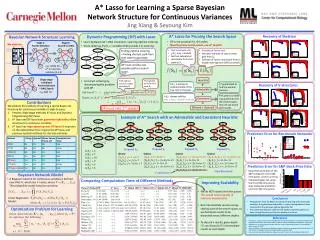
A* Lasso for Learning a Sparse Bayesian Network Structure for Continuous Variances

1. S0={} A* Lasso for Learning a Sparse Bayesian Network Structure for Continuous Variances S1={X1} S2={X2} S3={X3} S5 S5 S5 S5 S6 S6 S6 S6 S4 S4 S4 S4 S4={X1,X2} S5={X1,X3} S6={X2,X3} S7 S7 S7 S7 S7={X1,X2,X3} Jing Xiang & Seyoung Kim Recovery of V-structures A* Lasso for Pruning the Search Space Dynamic Programming (DP) with Lasso Bayesian Network Structure Learning We observe… X1 . . . X5 • DP is not practical for >20 nodes. • Need to prune search space, use A* search! • Learning Bayes net + DAG constraint = learning optimal ordering. • Given ordering, Pa(Xj) = variables that precede it in ordering. Stage 1: Parent Selection Stage 2: Search for DAG Sample 1 Sample 2 • Cost incurred so far. • g(Sk)only = Greedy • Fast but suboptimal • LassoScore from start state to Sk. Finding optimal ordering = finding shortest path from start state to goal state • Estimate of future cost • Heuristic estimate of cost to reach goal from Sk • Estimate of future LassoScore from Skto goal state (ignores DAG constraint). … X2 X2 X2 X1 X1 X1 Sample n X3 X3 X3 X4 X4 X4 DP must consider ALL possible paths in search space. e.g. L1MB, DP + A* for discrete variables [2,3,4] X5 X5 X5 Single stage combined Parent Selection + DAG Search Heuristic • Construct ordering by decomposing the problemwith DP. Find optimal score for first node Xj Find optimal score for nodes excluding Xj + h(Sk) is always an underestimate of the true cost to the goal. Recovery of Skeleton A* guaranteed to find the optimal solution. Admissible e.g. SBN [1] + h(Sk) always satisfies First path to a state is guaranteed to be the shortest path, thus we can prune other paths. Consistent Contributions = We address the problem of learning a sparse Bayes net structure for continuous variables in high-D space. Present single stage methods A* lasso and Dynamic Programming (DP) lasso. A* lasso and DP lasso both guarantee optimality of the structure for continuous variables. A* lasso has huge speed-up over DP lasso! It improves on the exponential time required by DP lasso, and previous optimal methods for discrete variables. Efficient + Optimal! DP must visit 2|V|states! ≠ Example of A* Search with an Admissible and Consistent Heuristic S0 S0 S0 S0 1 3 2 S2 S2 S2 S2 S3 S3 S3 S3 S1 S1 S1 S1 8 4 Prediction Error for Benchmark Networks 6 5 5 9 7 11 8 Expand S1 Expand S2 Expand S5 Expand S0 h(S1) = 4 h(S2) = 5 h(S3) = 10 h(S4) = 9 h(S5) = 5 h(S6) = 6 Queue {S0,S2}: f = 2+5= 7 {S0,S1,S5}: f = (1+4)+5= 10 {S0,S3}: f = 3+10= 13 {S0,S1,S4}: f = (1+5)+9= 15 Queue {S0,S1,S5,S7}: f = (1+4)+7= 12 {S0,S3}: f = 3+10= 13 {S0,S2,S6}: f = (2+5)+6= 13 {S0,S1,S4}: f = (1+5)+9= 15 Queue {S0,S1,S5}: f = (1+4)+5= 10 {S0,S3}: f = 3+10= 13 {S0,S2,S6}: f = (2+5)+6= 13 {S0,S1,S4}: f = (1+5)+9= 15 {S0,S2,S4}: f = (2+6)+9= 17 Queue {S0,S1}:f = 1+4= 5 {S0,S2}: f = 2+5= 7 {S0,S3}: f = 3+10= 13 Prediction Error for S&P Stock Price Data • Daily stock price data of 125 S&P companies over 1500 time points (1/3/07-12/17/12). • Estimated Bayes net using the first 1000 time points, then computed prediction errors on 500 time points. Goal Reached! Consistency! Bayesian Network Model • A Bayesian network for continuous variables is defined over DAGG, which has V nodes, where V = {X1, …, X|V|}. The probability model factorizes as below. Comparing Computation Time of Different Methods Improving Scalability • We do NOT naively limit the queue. This would reduce quality of solutions dramatically! • Best intermediate results occupy shallow part of the search space, so we distribute results to be discarded across different depths. • To discard kresults, given depth |V|, we discard k/|V| intermediate results at each depth. Linear Regression Model: Conclusions • Proposed A* lasso for Bayes net structure learning with continuous variables, this guarantees optimality + reduces computational time compared to the previous optimal algorithm DP. • Also presented heuristic scheme that further improves speed but does not significantly sacrifice the quality of solution. Optimization Problem for Learning References Huang et al. A sparse structure learning algorithm for Gaussian Bayesian network identification from high-dimensional data. IEEE Transactions on Pattern Analysis and Machine Intelligence, 35(6), 2013. Schmidt et al. Learning graphical model structure using L1-regularization paths. In Proceedings of AAAI, volume 22, 2007. Singh and Moore. Finding optimal Bayesian networks by dynamic programming. Technical Report 05-106, School of Computer Science, Carnegie Mellon University, 2005. Yuan et al. Learning optimal Bayesian networks using A* search. In Proceedings of AAAI, 2011.