Costs
Costs. “Cost” is not a simple concept. It is important to distinguish between four different types - fixed, variable, average and marginal .

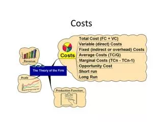
Costs
E N D
Presentation Transcript
Costs “Cost” is not a simple concept. It is important to distinguish between four different types - fixed, variable, average and marginal. What is the cost of an additional copy of Windows 2000? Multiply this by the total number sold. Would Bill Gates recover his investment at this price? Why not?
Costs & Profits • Profits = Revenues – Costs • Studied how revenues relate to output • Next we study how costs relate to output. • Then we can decide how profits vary with output and so what output levels are most profitable
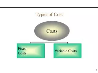
Cost Structures • First distinction: (1) fixed costs vs. (2) variable costs.
Fixed Costs • Independent of output level • examples: • cost of borrowed money • rental or mortgage payments on office/factory space • corporate HQ costs.
Variable Costs • Depend in some way on production levels within the organization • examples: • materials • some labor (depends on the contract) • power
Note that the line between fixed and variable costs is not always sharp and costs may be fixed for one analysis and variable for another - see the TV guide case.
TC = total cost, VC = variable cost, AC = average cost, etc. TC = FC + VC VC = VC(N) where N is the level of output AC = TC/N = FC/N + VC(N)/N
Variable costs linear in output: VC(N) = N Then AC = FC/N + is declining in N When are variable costs likely to rise proportionally to output? When more than proportionally? Less?
Variable cost proportional to output Average cost Large firms have cost advantage over smaller ones. FC/N +b b Output
Cost curves & Mergers • Falling average costs can provide impetus for mergers • Compaq-Hewlett Packard merger may be of this type, as were mergers of Chase and Chemical Bank. • Other motives may be in terms of product complementarity.
Variable costs quadratic in output: VC(N) = N + N2 Then AC = FC/N + + N This is -shaped as a function of N, falling for small N and then rising for large N.
Variable cost quadratic in output Average cost FC/N +b+gN b Output
Next Distinction • Marginal (or incremental) vs. • Average costs. • MC is probably the most import cost concept
Marginal Costs • MC is change in total cost as result of one unit change in output, TC(N) - TC(N-1) • Rate of change of total cost with respect to output: MC=DTC/DN =DFC/DN + DVC(N)/DN =DVC(N)/DN
Marginal Costs • MC depends only on variable costs • Shows cost impact of change in production – fixed costs have no relevance to cost consequence of output change
Variable cost proportional to output Average cost FC/N +b b Marginal cost Output
If MC < AC, then AC is falling If MC > AC, then AC is rising If MC = AC, then AC is constant What is the relationship between average and marginal costs?
A.k.a. Economies of scale Increasing returns to scale - AC falls as output rises. Decreasing returns - AC rises with output Constant returns - AC does not change with output. Returns to scale
Large fixed costs imply increasing returns - e.g., autos, telecoms, networks. Small fixed costs and VCs rising with o/p imply diminishing returns - e.g farming. Assembly operations usually show constant returns. Large fixed costs - economies of scale - make entry of competitors difficult. Returns to scale & cost structure
Autos - history of consolidation. Telecom networks prior to fiber optics - entry of MCI & Sprint into long distance after ATT deregulation Microsoft and Windows Scale economies & competition
Dynamic Changes inCosts--The Learning Curve • The learning curve measures the impact of worker’s experience on the costs of production. • It describes the relationship between a firm’s cumulative output and amount of inputs needed to produce a unit of output.
The Learning Curve • The horizontal axis measures the cumulative number of hours of machine tools the firm has produced • The vertical axis measures the number of hours of labor needed to produce each lot. Hours of labor per machine lot 10 8 6 4 2 0 10 20 30 40 50
Dynamic Changes inCosts--The Learning Curve • Observations 1) New firms may experience a learning curve, not economies of scale. 2) Older firms have relatively small gains from learning.
A B AC1 Learning C AC2 Economies ofScale Versus Learning Cost ($ per unit of output) Economies of Scale – reversible. Output
Dynamic Changes inCosts--The Learning Curve • The learning curve implies: 1) The labor requirement falls per unit. 2) Costs will be high at first and then will fall with learning.
The Learning Curve in Practice • The Empirical Findings • Study of 37 chemical products • Average cost fell 5.5% per year • For each doubling of plant size, average production costs fall by 11% (economies of scale) • For each doubling of cumulative output, the average cost of production falls by 27% (learning)
The Learning Curve in Practice • Other Empirical Findings • In the semi-conductor industry a study of seven generations of DRAM semiconductors from 1974-1992 found learning rates averaged 20%. • In the aircraft industry the learning rates are as high as 40%.
How do cost concepts relate to pricing? • Price should never be below marginal costs. • Can it make sense for price to be above marginal cost but below average costs? • Yes, but do not renew your investment in this case. This is a situation where you can stay in the business but it was a mistake to get into it in the first place. • In this case we cover variable costs but don’t recover fixed costs.
Breakeven: • Occurs at the output level at which total cost equals total revenue. • Let P(N) be the price at which N units can be sold. Then breakeven means: P(N) . N = FC + VC(N)
Total Cost = FC + VC(N) = FC + bN + c N2 MC = n + 2cN Costs Average total cost AC = FC/N + b + cN Price MC Output Breakeven
Study the elasticity of profits with respect to output Q. Let output change from Q to Q + Q, and profits from to + Intuition - must be greater, the greater are fixed costs. Leverage
Q = Q/Q Q The elasticity of profits with respect to output, denoted E ,Q, is: E ,Q = / This is the ratio of the proportional change in profits resulting from an output change to the proportional change in output causing it. If this number is 5, for example, it tells us that a 1% change in output leads to a 5% change in profits
Profit = PQ(revenue) - TC(total cost) = PQ - FC - VC Elasticity of with respect to Q: E,Q = (d/dQ)(Q/) d/dQ = P - (dVC/dQ) = P - MC E,Q = P-MC(Q/) P - MC = contribution to overhead or contribution margin
/Q = (PQ - AC*Q)/Q so (Q/) = 1/(P - AC) so E,Q = P-MC/P-AC “Operating leverage” MC = AC: E,Q = 1 MC < AC: E,Q > 1 MC > AC: E,Q < 1
Applications • Combine operating leverage with income elasticity of demand. • Firm has Op Lev of 5 and IED for products of 5. Then 1% rise in consumer income implies 5% rise in sales and 25% rise in profits – and vice versa for fall in demand • If Op Lev is 2 and IED is 2 then corresponding number is 4%.
Windows 95 Facts: • Development costs: $1.1 billion • Promotion costs: $1.2 billion • Variable costs: • zero for OEM use • very low for site licenses • $2-3 for retail sales • Retail price: $50 - $60 (to Microsoft)
Windows 95 Questions: • What is the average cost for various output levels? • What is the marginal cost? • What are the demand elasticities and the income elasticity? • What is the operating leverage? • What is the nature of competition? • Are there benefits to this product other than sales revenues?
Microsoft needed to sell 65 million units @ $35 to recover its fixed investment in the development and promotion of Windows. At $30, it had to sell 77 million units.
Price: averaging over range, let P = 35 Marginal cost: assume MC = 1, a constant Then for Output level Q, variable cost is VC = Q Fixed cost is FC = 2.3B (2.3 billion), so Total cost is TC = FC + VC = 2.3B + Q Operating Leverage for Microsoft Windows
2.3B Q P - MC P-AC 35 35 - 2.3B Q Average Cost: AC = TC/Q = 1 + Compute operating leverage using formula E,Q = E,Q = Q Q - 65M Multiply numerator and denominator by Q/35
Near the breakeven point, small fluctuations in output induce large fluctuations in profits. Thus if Q = 70 million copies, operating leverage is approximately 17 (a 1% increase in sales leads to a 17% jump in profits) If output expands to Q = 90 million copies, then operating leverage is 3.7A given fluctuation in sales induces a smaller proportionate increase in profits.
Cost Allocation • How should a multi-divisional company allocated corporate overhead costs between its divisions?
PC Computer Company (PCCC) has two operating divisions (1) Desk Top (DT) (2) Lap Top (LT)PCCC corporate overhead cost = $20m/year composed of: - interest on corporate debt - salaries of the President, CEO, and CFO - corporate promotional costs - central office costs (accounting, HR, management, etc.)
Divisional costs DT’s division-specific fixed costs are $50m/year (equipment and fixed labor) and variable costs are $1,000/machine (components, labor, testing) DT sells machines for $1,500 each. LT’s division-specific fixed costs are $50m/year and variable costs are $1,500 per machine, which sell for $2,000 each.
Consider the following questions: • At what output level does each division cover its division specific costs? • How does each division’s contribution to corporate overheads and profits change with output once it exceeds the output level which answers (1) • When does PCCC as a whole make profits?
Answers: • DT will break even at sales of 100,000 relative to divisional costs. • LT will also break even at 100,000. • We will need an extra 40,000 units to cover corporate overheads of $20m - i.e. a total sales of 240,000. • The make-up of this 40,000 sales total does not matter.
The CFO decides to allocate overheads to DT and LT, $10m/year to each. The CEO then decides to close down any division which is not covering division-specific costs plus its allocated overhead. Evaluate this policy. What conclusion can you draw about the appropriate test of a division’s financial performance?