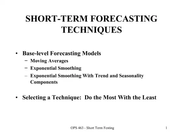
SHORT-TERM FORECASTING TECHNIQUES
OPS 463 - Short Term Fcsting. 2. BASE-LEVEL FORECASTING MODELS. Assume absence of trend and seasonalitySeparate base-level from randomnessFt -- Forecast for period tAt -- Actual sales for period tBt -- Base level component for period tet -- Random element for period t. OPS 463 - Short

SHORT-TERM FORECASTING TECHNIQUES
E N D
Presentation Transcript
1. OPS 463 - Short Term Fcsting 1 SHORT-TERM FORECASTING TECHNIQUES
Base-level Forecasting Models
Moving Averages
Exponential Smoothing
Exponential Smoothing With Trend and Seasonality Components
Selecting a Technique: Do the Most With the Least
2. OPS 463 - Short Term Fcsting 2 BASE-LEVEL FORECASTING MODELS Assume absence of trend and seasonality
Separate base-level from randomness
Ft -- Forecast for period t
At -- Actual sales for period t
Bt -- Base level component for period t
et -- Random element for period t
3. OPS 463 - Short Term Fcsting 3 BASE-LEVEL FORECASTING MODELS Example: tricycle sales at Bikes-R-Us
Actual July Sales: 105
�True� Base level for July: 100
Random spike for July: 105-100 = 5
Assumption: At = Bt + et ; [105 = 100 + 5]
Practical implications for forecasting:
Step 1: Smooth randomness out of At to estimate Bt
Step 2: Set Ft+1 = Bt
4. OPS 463 - Short Term Fcsting 4 NA�VE METHOD No smoothing of data
Step 1: Bt = At
Step 2: Ft+1 = Bt
5. OPS 463 - Short Term Fcsting 5 NA�VE METHOD No smoothing of data
Step 1: Bt = At
Step 2: Ft+1 = Bt
6. OPS 463 - Short Term Fcsting 6 NA�VE METHOD No smoothing of data
Step 1: Bt = At
Step 2: Ft+1 = Bt
7. OPS 463 - Short Term Fcsting 7 NA�VE METHOD No smoothing of data
Step 1: Bt = At
Step 2: Ft+1 = Bt
8. OPS 463 - Short Term Fcsting 8 SIMPLE MOVING AVERAGE Smoothes out randomness by averaging positive and negative random elements over several periods
n -- number of periods
Step 1:
Step 2: Ft+1 = Bt
9. OPS 463 - Short Term Fcsting 9 SIMPLE MOVING AVERAGE Smoothes out randomness by averaging positive and negative random elements over several periods
n -- number of periods
Step 1:
Step 2: Ft+1 = Bt
10. OPS 463 - Short Term Fcsting 10 SIMPLE MOVING AVERAGE Smoothes out randomness by averaging positive and negative random elements over several periods
n -- number of periods
Step 1:
Step 2: Ft+1 = Bt
11. OPS 463 - Short Term Fcsting 11 SIMPLE MOVING AVERAGE Smoothes out randomness by averaging positive and negative random elements over several periods
n -- number of periods
Step 1:
Step 2: Ft+1 = Bt
12. OPS 463 - Short Term Fcsting 12 WEIGHTED MOVING AVERAGE Same idea as SMA, but less smoothing: more weight on recent sales data
n -- number of periods
ai � weight applied to period t-i+1
Step 1:
Step 2: Ft+1 = Bt
13. OPS 463 - Short Term Fcsting 13 WEIGHTED MOVING AVERAGE Same idea as SMA, but less smoothing: more weight on recent sales data
n -- number of periods
ai � weight applied to period t-i+1
Step 1:
Step 2: Ft+1 = Bt
14. OPS 463 - Short Term Fcsting 14 WEIGHTED MOVING AVERAGE Same idea as SMA, but less smoothing: more weight on recent sales data
n -- number of periods
ai � weight applied to period t-i+1
Step 1:
Step 2: Ft+1 = Bt
15. OPS 463 - Short Term Fcsting 15 WEIGHTED MOVING AVERAGE Same idea as SMA, but less smoothing: more weight on recent sales data
n -- number of periods
ai � weight applied to period t-i+1
Step 1:
Step 2: Ft+1 = Bt
16. OPS 463 - Short Term Fcsting 16 EXPONENTIAL SMOOTHING (I) Simpler equation, equivalent to WMA
a � exponential smoothing parameter (0< a<1)
Step 1:
Step 2: Ft+1 = Bt
17. OPS 463 - Short Term Fcsting 17 EXPONENTIAL SMOOTHING (I) Simpler equation, equivalent to WMA
a � exponential smoothing parameter (0< a<1)
Step 1:
Step 2: Ft+1 = Bt
18. OPS 463 - Short Term Fcsting 18 EXPONENTIAL SMOOTHING (I) Simpler equation, equivalent to WMA
a � exponential smoothing parameter (0< a<1)
Step 1:
Step 2: Ft+1 = Bt
19. OPS 463 - Short Term Fcsting 19 EXPONENTIAL SMOOTHING (I) Simpler equation, equivalent to WMA
a � exponential smoothing parameter (0< a<1)
Step 1:
Step 2: Ft+1 = Bt
20. OPS 463 - Short Term Fcsting 20 EXPONENTIAL SMOOTHING (I) Simpler equation, equivalent to WMA
a � exponential smoothing parameter (0< a<1)
Step 1:
Step 2: Ft+1 = Bt
21. OPS 463 - Short Term Fcsting 21 EXPONENTIAL SMOOTHING (II) A higher smoothing parameter means less smoothing and a more reactive forecast
22. OPS 463 - Short Term Fcsting 22 E.S. WITH TREND Assumes existence of Trend and Base Level
Tt � Trend component in period t
a � Base-level smoothing parameter (0< a<1)
b � Trend smoothing parameter (0< b<1)
Step 1:
Step 2: Ft+1 = Bt + Tt
23. OPS 463 - Short Term Fcsting 23 E.S. WITH TREND Assumes existence of Trend and Base Level
Tt � Trend component in period t
a � Base-level smoothing parameter (0< a<1)
b � Trend smoothing parameter (0< b<1)
Step 1:
Step 2: Ft+1 = Bt + Tt
24. OPS 463 - Short Term Fcsting 24 E.S. WITH TREND Assumes existence of Trend and Base Level
Tt � Trend component in period t
a � Base-level smoothing parameter (0< a<1)
b � Trend smoothing parameter (0< b<1)
Step 1:
Step 2: Ft+1 = Bt + Tt
25. OPS 463 - Short Term Fcsting 25 E.S. WITH TREND Assumes existence of Trend and Base Level
Tt � Trend component in period t
a � Base-level smoothing parameter (0< a<1)
b � Trend smoothing parameter (0< b<1)
Step 1:
Step 2: Ft+1 = Bt + Tt
26. OPS 463 - Short Term Fcsting 26 E.S. WITH TREND Assumes existence of Trend and Base Level
Tt � Trend component in period t
a � Base-level smoothing parameter (0< a<1)
b � Trend smoothing parameter (0< b<1)
Step 1:
Step 2: Ft+1 = Bt + Tt
27. OPS 463 - Short Term Fcsting 27 E.S. WITH TREND Assumes existence of Trend and Base Level
Tt � Trend component in period t
a � Base-level smoothing parameter (0< a<1)
b � Trend smoothing parameter (0< b<1)
Step 1:
Step 2: Ft+1 = Bt + Tt
28. OPS 463 - Short Term Fcsting 28 E.S. WITH TREND & SEASONS St � Seasonality component in period t
L � Number of seasons in a year
g � Seasonality smoothing parameter (0< g<1)
Step 1:
Step 2: Ft+1 = (Bt +Tt )St-L+1
29. OPS 463 - Short Term Fcsting 29 E.S. WITH TREND & SEASONS St � Seasonality component in period t
L � Number of seasons in a year
g � Seasonality smoothing parameter (0< g<1)
Step 1:
Step 2: Ft+1 = (Bt +Tt )St-L+1
30. OPS 463 - Short Term Fcsting 30 E.S. WITH TREND & SEASONS St � Seasonality component in period t
L � Number of seasons in a year
g � Seasonality smoothing parameter (0< g<1)
Step 1:
Step 2: Ft+1 = (Bt +Tt )St-L+1
31. OPS 463 - Short Term Fcsting 31 E.S. WITH TREND & SEASONS St � Seasonality component in period t
L � Number of seasons in a year
g � Seasonality smoothing parameter (0< g<1)
Step 1:
Step 2: Ft+1 = (Bt +Tt )St-L+1
32. OPS 463 - Short Term Fcsting 32 E.S. WITH TREND & SEASONS St � Seasonality component in period t
L � Number of seasons in a year
g � Seasonality smoothing parameter (0< g<1)
Step 1:
Step 2: Ft+1 = (Bt +Tt )St-L+1
33. OPS 463 - Short Term Fcsting 33 E.S. WITH TREND & SEASONS St � Seasonality component in period t
L � Number of seasons in a year
g � Seasonality smoothing parameter (0< g<1)
Step 1:
Step 2: Ft+1 = (Bt +Tt )St-L+1
34. OPS 463 - Short Term Fcsting 34 E.S. WITH TREND & SEASONS St � Seasonality component in period t
L � Number of seasons in a year
g � Seasonality smoothing parameter (0< g<1)
Step 1:
Step 2: Ft+1 = (Bt +Tt )St-L+1
35. OPS 463 - Short Term Fcsting 35 E.S. WITH TREND & SEASONS St � Seasonality component in period t
L � Number of seasons in a year
g � Seasonality smoothing parameter (0< g<1)
Step 1:
Step 2: Ft+1 = (Bt +Tt )St-L+1
36. OPS 463 - Short Term Fcsting 36 E.S. WITH TREND & SEASONS St � Seasonality component in period t
L � Number of seasons in a year
g � Seasonality smoothing parameter (0< g<1)
Step 1:
Step 2: Ft+1 = (Bt +Tt )St-L+1
37. OPS 463 - Short Term Fcsting 37 E.S. WITH TREND & SEASONS St � Seasonality component in period t
L � Number of seasons in a year
g � Seasonality smoothing parameter (0< g<1)
Step 1:
Step 2: Ft+1 = (Bt +Tt )St-L+1
38. OPS 463 - Short Term Fcsting 38 E.S. WITH TREND & SEASONS St � Seasonality component in period t
L � Number of seasons in a year
g � Seasonality smoothing parameter (0< g<1)
Step 1:
Step 2: Ft+1 = (Bt +Tt )St-L+1
39. OPS 463 - Short Term Fcsting 39 FORECASTING MORE THAN ONE PERIOD AHEAD m � # periods ahead to be forecast
Base level forecasts: Ft+m = Bt
Forecasts with trend: Ft+m = Bt +mTt
Forecasts with seasonality: Ft+m = (Bt +mTt )St-L+m
40. OPS 463 - Short Term Fcsting 40 SELECTING A TECHNIQUE Ockham's razor -- use the simplest possible model or theory (William of Ockham, 1300-1349, England)
1) Determine type of technique which is appropriate (i.E., Base-level, trend, etc.)
2) Select a group of competing techniques which satisfy condition (1)
3) Select a set of data as a test set
4) Simulate forecasts for this set of data using all techniques from (2)
5) Pick the technique with the best combination of MAD/MAPE and Bias