The M/M/1 Queue
The M/M/1 Queue. The easiest queue to analyse. Distributed Probability. If we have a variable which can have any value over a range, (not simply integer values) we must talk about its probability distribution

The M/M/1 Queue
E N D
Presentation Transcript
The M/M/1 Queue The easiest queue to analyse
Distributed Probability • If we have a variable which can have any value over a range, (not simply integer values) we must talk about its probability distribution • If the probability distribution function is f(x), then the probability that the value of x is between x1 and x1 + dx is f(x1)dx
Distributed Probability • The probability x is between x1 and x2 is • If x1 and x2 are the limits placed on x then we also have
Inter-arrival Time • During a Poisson process, the packets will arrive at intervals along the time line. The period between two successive arrivals can have any value along a continuum • This value will be statistically distributed
Inter-arrival Time • tis an inter-arrival time Arrivals t time
Inter-arrival Time • Probability next packet arrives after t = x is e-lx (exponential or Poisson distribution) • So probability next packet arrives before t = x is 1 – e-lx
Inter-arrival Time • Now, let f(u) be the probability density for the inter-arrival time • Then the probability that an inter-arrival time is less than x is • But this is just the probability that the next packet arrives before t = x
Inter-arrival Time • Therefore • Differentiating both sides w.r.t x gives us • f(x) = le-lx
Inter-arrival Time f(t) • This result tells us that an inter-arrival time is more likely to be about x1 (short) than x2 (long) for any l dt dt t x1 x2
Service Times • We will assume that the times taken to service packets are also exponentially distributed, with rate parameter, m • That is, while there are any packets in the queue, including the packet in service, the service completion times also give a Poisson process
Service Times • In some situations, this is a reasonable approximation, eg IP packets, which have variable size • But in ATM systems, the cells are all the same size, and mostly, one cell will be served from each queue at each cell time
Kendall Notation • A queuing system with a Markov (Poisson) arrival process, Markov service process, s servers and K places in the buffer is called a M/M/s/K system in the Kendal notation. • Usually the last part is omitted giving M/M/1 for our queue
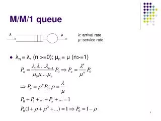
M/M/1 Queue • The important variable (or state) in a queuing system is n, the number of packets in the queue • The important parameter is pn, the probability that we will find the queue with n members • l and m are the arrival and service rates
M/M/1 Queue l l l l l l … • The state diagram gives a good picture of the M/M/1 queue • The state, n, can never be less than 0 … 0 1 2 n-1 n n+1 m m m m m m
M/M/1 Queue • When the queue is in any state, n, the average rate of incoming packets is l, and the average rate of service is m • The probabilities that it will be in states, n and n + 1 are pn and pn+1 • On the average, the number of transitions from n to n+1 will equal the number from n+1 to n
M/M/1 Queue • This means that lpn = mpn+1 • We define r = l/m • Then pn+1 = rpn • We can apply this formula any number of times, starting with n = 0 to give • pn = rnp0 • Now we need to find p0
M/M/1 Queue • If we add all the probabilities, they must total 1.0 • for r < 1 • That is, p0 = 1 - r
M/M/1 Queue pn 0.5 0.4 0.3 0.2 0.1 0 • Probabilities for r = 0.5 • This is called a “geometric distribution” n 0 1 2 3
M/M/1 Queue • Probability that n = 0 is 1 – r • Therefore probability that a queue exists is simply r • Since r is the ratio of the average incoming rate to the average service rate, it is often called the “utilisation” (cf utilisation of a link)
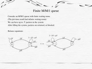
Finite M/M/1 Queue • If there is only space for N packets in the queue, then clearly N is an upper limit on n, • Any packet which arrives while n = N cannot be stored, and will be lost • In queuing theory, this is called “blocking”
Finite M/M/1 Queue • The state model of the infinite buffer will be modified so that Pn = 0 for n > N • So
Finite M/M/1 Queue • This gives • And • What does this mean, physically? How do the probabilities we calculate determine what happens in a queue?
Physical Picture • Queue for r = 0.6 over 1000 time steps
Probabilities • Probabilities from last example of queue • Last column is calculated (theoretical for r = 0.6)
Blocking Probability • An important design criterion is the blocking probability of a queuing system • Would we be happy to lose one packet in 100?, 1000? 1000,000? • How much extra buffer space must we put in to achieve these figures?
Blocking Probability • If a queue is full when a packet arrives, it will be discarded, or “blocked” • So the probability that a packet is blocked is exactly the same as the probability that the queue is full • That is, PB = pN
Blocking Probability • Schwartz has this useful diagram to describe throughput and blocking l = load Queue • = throughput = l(1-PB) lPB
Blocking Probability • From this diagram we see that, for any queue • g = l(1 – PB) = m(1 – p0) • For a M/M/1 queue, we have p0 from before. If we substitute into this equation we will get the same formula for PB (Try it yourself)
Design of Blocking System • If • Then we can find the necessary buffer length, if we know r • The next slide tabulates the buffer size for combinations of PB and r • (Check these figures yourself)
Required Buffer Size • Comment: • For low utilisation, r, the requirements on the buffer are not heavy, even if we lose only one packet in a million • When the utilisation is 0.9, then we need 44 buffer spaces, even if we lose one in 1000
Required Buffer Size • 0.9 is a very high utilisation. • It is more usual to try to run a system with utilisation of 0.7 at the maximum
Mean Queue Length • The average queue length is important since it lets us know what time delay to expect because of the time a packet spends waiting in a queue
Mean Queue Length • Queue length is 3 for r = 0.75, but goes to 9 for r = 0.9 and to 19 for r = 0.95 • When r is less than 0.5, the average queue length is less than 1.0 • There is little delay (or buffer space required) when r is low
Average Time Delay • For an infinite buffer, the expected time delay is • Of this time, a period, 1/m is spent actually being serviced, the rest is spent waiting in the queue
Average Service Time • Question: At what utilisation, does a packet spend as much time waiting in the queue as it does being served (transmitted)? • For this to happen • Or r = 0.5