Understanding Little's Queuing Formula: Application in Steady-State Conditions
This document explores Little's queuing formula, applicable in various steady-state conditions, independently of the number of servers, queue discipline, interarrival time distribution, and service time distribution. It provides practical insights through the example of a fast-food establishment, analyzing key performance metrics such as service rates, customer waiting times, and system costs. Additionally, it discusses different types of costs associated with queuing systems, including loss of goodwill, waiting time costs, and space costs, guiding readers on optimizing queuing systems for efficiency.

Understanding Little's Queuing Formula: Application in Steady-State Conditions
E N D
Presentation Transcript
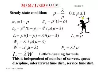
M / M / 1 / GD / /(Section 4) Steady-state condition: Little’s queuing formula This is independent of number of servers, queue discipline, interarrival time dist., service time dist. IE 417, Chap 22, April 99
Burger-417 Fast-Food = 45#/hr = 0.75#/min = 60#/hr = 1#/min Based on solution on web. 1 teller 1 teller & cashier 2 tellers = 1 = 1.25 = 1 Lq# 2.25 0.9 0.12 L # 3 1.5 0.87 Wqmin 3 1.2 0.16 W min 4 2 1.16 0.75 0.6 0.38 0.25 0.4 0.45 Pw 0.75 0.6 0.20 P(j 5) 0.24 0.08 0.01 1 IE 417, Chap 22, May 99
Different Types of Costs in Queuing Systems Loss in goodwill = ($/part) C Waiting time = ($/unit time) Cost of space = ($/part) Lq Loss of customer = ($/part) IE 417, Chap 22, April 99
M / M / 1 / GD / C /(Section 5) For j = 1, …., C For j = 0, …., C For j = C+1, …., IE 417, Chap 22, May 99
M / M / S / GD / /(Section 6) Steady-state condition: For j = 1, 2, …, S For j = S+1, S+2, …, Probability that an arriving unit has to wait: Table 6 page 1088 IE 417, Chap 22, May 99
M / M / S / GD / /(Section 6) Cont. IE 417, Chap 22, May 99