Monte Carlo Simulations in Matlab
220 likes | 769 Vues
Jake Blanchard University of Wisconsin Spring 2006. Monte Carlo Simulations in Matlab. Introduction. Monte Carlo approaches use random sampling to simulate physical phenomena

Monte Carlo Simulations in Matlab
E N D
Presentation Transcript
Jake Blanchard University of Wisconsin Spring 2006 Monte Carlo Simulations in Matlab
Introduction • Monte Carlo approaches use random sampling to simulate physical phenomena • They have been used to simulate particle transport, risk analysis, reliability of components, molecular modeling, and many other areas
An Example – Beam Bending • Consider a cantilever beam with a load (F) applied at the end • Assume that the diameter (d) of the beam cross section, the load (F), and the elastic modulus (E) of the beam material vary from beam to beam (L is constant – 10 centimeters) • We need to know the character of the variations in the displacement () of the end of the beam
Cantilever Beam F d
Analysis • If F is the only random variable and F has, for example, a lognormal distribution, then the deflection will also have a lognormal distribution • But if several variables are random, then the analysis is much more complication
Approach • Assume/determine a distribution function to represent all input variables • Sample each (independently) • Calculate the deflection from the formula • Repeat many times to obtain output distribution
Our Case Study • Assume E, d, and F are random variables with uniform distributions
Script to calculate one value length=0.1 force=1000+50*rand(1) diameter=0.01+rand(1)*0.001 modulus=200e9+rand(1)*10e9 inertia=pi*diameter^4/64 displacement=force*length^3/3/modulus/inertia
Script to calculate many values (using “for” loop) length=0.1 nsamples=100000 for i=1:nsamples force=1000+50*rand(1); diameter=0.01+rand(1)*0.001; modulus=200e9+rand(1)*10e9; inertia=pi*diameter^4/64; displacement(i)=force*length^3/3/modulus/inertia; end
Script to calculate many values (direct approach) length=0.1 nsamples=100000 force=1000+50*rand(nsamples,1); diameter=0.01+rand(nsamples,1)*0.001; modulus=200e9+rand(nsamples,1)*10e9; inertia=pi*diameter.^4/64; displacement=force.*length^3/3./modulus./inertia;
Performance comparison • The direct approach is much faster • For 100,000 samples the loop takes about 3.9 seconds and the direct approach takes about 0.15 seconds (a factor of almost 30 • I used the “tic” and “toc” commands to time these routines
Looking at results • Mean • Standard deviation • histogram min(displacement) max(displacement) mean(displacement) std(displacement) hist(displacement, 50)