Lecture 12 Monte Carlo Simulations
580 likes | 1.01k Vues
Lecture 12 Monte Carlo Simulations. Useful web sites: http://kurslab-atom.fysik.lth.se/FED4Medopt/MonteCarloSim.pdf http://omlc.ogi.edu/classroom/ece532/class4/index.html. Introduction. Monte Carlo method

Lecture 12 Monte Carlo Simulations
E N D
Presentation Transcript
Lecture 12Monte Carlo Simulations Useful web sites: http://kurslab-atom.fysik.lth.se/FED4Medopt/MonteCarloSim.pdf http://omlc.ogi.edu/classroom/ece532/class4/index.html
Introduction Monte Carlo method • Simulates photon transport in turbid medium such as tissue, that contains absorption and scattering • This model is based on a random walk, where a photon or a photon package is traced through the tissue until it exits or until it gets entirely absorbed • The method is based on a set of rules that govern the movement of the photon in tissue (transport equation); the 2 key decisions: 1) the mean free path for an absorption or scattering event 2) the scattering angle
Introduction Monte Carlo method Incident Light Emitted Light Absorption Event
Introduction Input - photons • The rules of photon propagation are expressed as probability distributions (for incremental steps) • The method is statistical in nature and requires the propagation of a large number of photons • Computational time is proportional to the number of photons launched in the simulation (typically, 1E6); number of photons determine precision
I. Introduction Output r Large Number of Photons Reflectance z Fluence Transmission
I. Introduction Assumptions • The simulations treat photons as neutral particles rather than as a wave phenomenon • It is assumed that the photons are multiply scattered by tissues • Therefore, phase and polarization are assumed to be randomized and can be ignored
I. Introduction Limitations • The Monte Carlo method is based on macroscopic optical properties that are assumed to extend uniformly over the tissue volume • Cannot handle small heterogeneities such as photon transport in cells or organelles • Significant computational time; not ideal for real-time analysis • Does not provide intuition on the dependence of reflectance on optical properties
Monte Carlo Simulations • Why? • Perform simulations for conditions under which the accuracy of the diffusion approximation is limited • Simulate more complicated tissue geometries (multilayer media) • Simulate more complicated light illumination geometries (collimated, angled, Gaussian beam illumination)
II. Selecting Variables I. Selecting step size II. Selecting direction: deflection angle azimuthal angle
II. Selecting the Variables The variables that govern Monte Carlo • The mean free path for an absorption or scattering event Step size (function of ma and ms) • The scattering angle Deflection angle, q (function of anisotropy, g) Azimuthal angle, y • Random number generators will be used for the selection of step size, deflection angle and azimuthal angle for sampling from known probability density functions
II. Selecting the Variables The variables that govern Monte Carlo
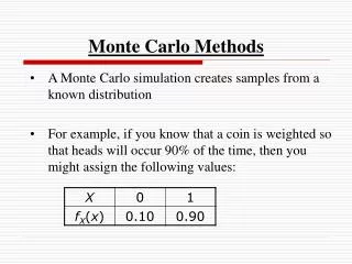
II. Selecting the Variables Basis for the Monte Carlo method • The Monte Carlo method as its name implies (“throwing the dice”) relies on the random sampling of a probability density function based on a computer generated random number • Need to understand definitions for probability density functions and probability distributions
II. Selecting the Variables Random variable, “x” A probability density function is a function defined on a continuous interval so that the area under the curve described by the function is unity The probability density function p(x) for some random variable, x, defines the distribution of x over the interval a<x<b, such that:
II. Selecting the Variables Random variable, “x” • The probability that x will fall in the interval [a,x1] such that a < x< x1, is given by a probability distribution function, F(x1) which is defined by:
II. Selecting the Variables Random variable, “x”
II. Selecting the Variables Random Numbers • Now we want to utilize a uniform random number generator of the computer to generate a random variable, rnd between 0 and 1 • The uniform probability density function (for the random number) will be mapped to a specific probability density function p(x) corresponding to step size, deflection angle and azimuthal angle
II. Selecting the Variables Random number, rnd • Now apply the same logic to the probability density function for a random number, rnd • The probability density function for a random number, rnd is a constant over [0,1]:
II. Selecting the Variables Random number, rnd • The probability that rnd will fall in the interval [0, rnd1] such that 0 < rnd<rnd1, is given by the probability distribution function, F(rnd1) which is defined by:
II. Selecting the Variables Random number, rnd
II. Selecting the Variables Relationship between x and rnd • The key to the Monte Carlo selection of x using rnd is to equate the probability that rnd is in the interval [0, rnd1] with the probability that x is in the interval [a,x1] • In other words, we can equate F(x) to F(rnd); i.e., we are equating the shaded areas under the curves
II. Selecting the Variables Random number, rnd
II. Selecting the Variables Basic equation • For generality, we replace the variables, rnd1 and x1 by the continuous variables, rnd and x: • This is the basic equation for sampling x from p(x) using a randomly generated number, rnd over the interval [0,1]
II. Selecting the Variables Random Numbers • Need pdfs for step size, deflection angle and azimuthal angle • Need to relate rnd to pdf using the transformation expression • Express step size, deflection angle and azimuthal angle in terms of rnd
II. Selecting the Variables Three equations • Step size • Deflection angle • Azimuthal angle
II. Selecting the Variables The known parameters Incident Light Emitted Light nm Absorption Event ma (l), ms (l), g(l), nt
III. Photon Propagation Initializing and launching the photon • Each photon is initially assigned a weight, W equal to unity, before it is injected into the tissue at the origin • If there is a mismatched boundary between the outside medium (m) and tissue (t), then specular reflectance will occur (Fresnel law): • The resulting photon weight, W is decreased to:
III. Photon Propagation Generating the step size • The computer’s random number generator yields a random variable, rnd, in the interval [0,1] and the sampling of the step size, s is given by:
III. Photon Propagation Photon absorption • Once the photon has taken a step, some attenuation of the photon weight due to absorption must occur; the amount of deposited photon weight, DQ is: • The new photon weight, W is:
III. Photon Propagation Terminating a photon • A technique called Roulette is used to terminate the photon when W < Wthreshold • This technique gives the photon one chance in m of surviving with a weight, mW. • This is also carried out using a random number generator.
III. Photon Propagation Change photon direction • If the photon survived, it is ready to be scattered • Photon deflection angle, q equals cos-1(m) (Here m is related to anisotropy) • Photon azimuthal angle is y • Next the new trajectory of the photon (mx’, my’, mz’), can be calculated from the old trajectory • Where, mx’, my’, and mz’ are the direction cosines specified by taking the angle that the photon direction makes with each axis
II. Selecting the Variables Three equations • Step size • Deflection angle • Azimuthal angle
III. Photon Propagation Internal reflection or escape • The internal reflectance is also calculated using Fresnel’s law • A fraction, 1-R(q) of the current photon weight successfully escapes the tissue as observable reflectance and updates the total reflectance • A fraction R(q) of the current photon weight is internally reflected. The new photon weight is: R(q)W
