Gene Prediction: Frequency-Based DNA Modeling for Coding Regions
390 likes | 527 Vues
This text explores the computational challenge of gene prediction, which involves identifying the start and end positions of genes within a genome. It discusses the fundamental concepts of genes as sequences of nucleotides coding for proteins and describes a frequency-based model that leverages the GC content in DNA sequences. By analyzing the distribution of GC and AT pairs between known coding and non-coding regions, the model predicts coding sequences. This approach provides insights into the differences between coding and non-coding DNA regions and highlights its practical applications in genomics.

Gene Prediction: Frequency-Based DNA Modeling for Coding Regions
E N D
Presentation Transcript
Probabilistic sequence modeling I: frequency and profiles Haixu Tang School of Informatics
Genome and genes • Genome: an organism’s genetic material (Car encyclopedia) • Gene: a discrete units of hereditary information located on the chromosomes and consisting of DNA. (Chapters to make components of a car, or to use and drive a car).
Gene Prediction: Computational Challenge aatgcatgcggctatgctaatgcatgcggctatgctaagctgggatccgatgacaatgcatgcggctatgctaatgcatgcggctatgcaagctgggatccgatgactatgctaagctgggatccgatgacaatgcatgcggctatgctaatgaatggtcttgggatttaccttggaatgctaagctgggatccgatgacaatgcatgcggctatgctaatgaatggtcttgggatttaccttggaatatgctaatgcatgcggctatgctaagctgggatccgatgacaatgcatgcggctatgctaatgcatgcggctatgcaagctgggatccgatgactatgctaagctgcggctatgctaatgcatgcggctatgctaagctgggatccgatgacaatgcatgcggctatgctaatgcatgcggctatgcaagctgggatcctgcggctatgctaatgaatggtcttgggatttaccttggaatgctaagctgggatccgatgacaatgcatgcggctatgctaatgaatggtcttgggatttaccttggaatatgctaatgcatgcggctatgctaagctgggaatgcatgcggctatgctaagctgggatccgatgacaatgcatgcggctatgctaatgcatgcggctatgcaagctgggatccgatgactatgctaagctgcggctatgctaatgcatgcggctatgctaagctcatgcggctatgctaagctgggaatgcatgcggctatgctaagctgggatccgatgacaatgcatgcggctatgctaatgcatgcggctatgcaagctgggatccgatgactatgctaagctgcggctatgctaatgcatgcggctatgctaagctcggctatgctaatgaatggtcttgggatttaccttggaatgctaagctgggatccgatgacaatgcatgcggctatgctaatgaatggtcttgggatttaccttggaatatgctaatgcatgcggctatgctaagctgggaatgcatgcggctatgctaagctgggatccgatgacaatgcatgcggctatgctaatgcatgcggctatgcaagctgggatccgatgactatgctaagctgcggctatgctaatgcatgcggctatgctaagctcatgcgg
Gene Prediction: Computational Challenge aatgcatgcggctatgctaatgcatgcggctatgctaagctgggatccgatgacaatgcatgcggctatgctaatgcatgcggctatgcaagctgggatccgatgactatgctaagctgggatccgatgacaatgcatgcggctatgctaatgaatggtcttgggatttaccttggaatgctaagctgggatccgatgacaatgcatgcggctatgctaatgaatggtcttgggatttaccttggaatatgctaatgcatgcggctatgctaagctgggatccgatgacaatgcatgcggctatgctaatgcatgcggctatgcaagctgggatccgatgactatgctaagctgcggctatgctaatgcatgcggctatgctaagctgggatccgatgacaatgcatgcggctatgctaatgcatgcggctatgcaagctgggatcctgcggctatgctaatgaatggtcttgggatttaccttggaatgctaagctgggatccgatgacaatgcatgcggctatgctaatgaatggtcttgggatttaccttggaatatgctaatgcatgcggctatgctaagctgggaatgcatgcggctatgctaagctgggatccgatgacaatgcatgcggctatgctaatgcatgcggctatgcaagctgggatccgatgactatgctaagctgcggctatgctaatgcatgcggctatgctaagctcatgcggctatgctaagctgggaatgcatgcggctatgctaagctgggatccgatgacaatgcatgcggctatgctaatgcatgcggctatgcaagctgggatccgatgactatgctaagctgcggctatgctaatgcatgcggctatgctaagctcggctatgctaatgaatggtcttgggatttaccttggaatgctaagctgggatccgatgacaatgcatgcggctatgctaatgaatggtcttgggatttaccttggaatatgctaatgcatgcggctatgctaagctgggaatgcatgcggctatgctaagctgggatccgatgacaatgcatgcggctatgctaatgcatgcggctatgcaagctgggatccgatgactatgctaagctgcggctatgctaatgcatgcggctatgctaagctcatgcgg
Gene Prediction: Computational Challenge aatgcatgcggctatgctaatgcatgcggctatgctaagctgggatccgatgacaatgcatgcggctatgctaatgcatgcggctatgcaagctgggatccgatgactatgctaagctgggatccgatgacaatgcatgcggctatgctaatgaatggtcttgggatttaccttggaatgctaagctgggatccgatgacaatgcatgcggctatgctaatgaatggtcttgggatttaccttggaatatgctaatgcatgcggctatgctaagctgggatccgatgacaatgcatgcggctatgctaatgcatgcggctatgcaagctgggatccgatgactatgctaagctgcggctatgctaatgcatgcggctatgctaagctgggatccgatgacaatgcatgcggctatgctaatgcatgcggctatgcaagctgggatcctgcggctatgctaatgaatggtcttgggatttaccttggaatgctaagctgggatccgatgacaatgcatgcggctatgctaatgaatggtcttgggatttaccttggaatatgctaatgcatgcggctatgctaagctgggaatgcatgcggctatgctaagctgggatccgatgacaatgcatgcggctatgctaatgcatgcggctatgcaagctgggatccgatgactatgctaagctgcggctatgctaatgcatgcggctatgctaagctcatgcggctatgctaagctgggaatgcatgcggctatgctaagctgggatccgatgacaatgcatgcggctatgctaatgcatgcggctatgcaagctgggatccgatgactatgctaagctgcggctatgctaatgcatgcggctatgctaagctcggctatgctaatgaatggtcttgggatttaccttggaatgctaagctgggatccgatgacaatgcatgcggctatgctaatgaatggtcttgggatttaccttggaatatgctaatgcatgcggctatgctaagctgggaatgcatgcggctatgctaagctgggatccgatgacaatgcatgcggctatgctaatgcatgcggctatgcaagctgggatccgatgactatgctaagctgcggctatgctaatgcatgcggctatgctaagctcatgcgg Gene!
Gene Prediction: Computational Challenge • Gene: A sequence of nucleotides coding for protein • Gene Prediction Problem: Determine the beginning and end positions of genes in a genome
A simple model for gene prediction: frequency-based DNA modeling • DNA is a double strand molecule • G-C pair strong • A-T pair weak • Coding regions often have higher GC content than non-coding regions
Frequency-based DNA modeling of coding vs. non-coding regions • To predict coding regions in an organism (e.g. human), collect a set of known coding and non-coding DNA sequences from this organism (training set) • Compute the frequency distribution of GC and AT pairs in coding and non-coding regions, respectively: F(fGC|c), F(fAT|c)=1-F(fGC|c); F(fGC|nc), F(fAT|nc)=1- F (fGC|nc);
A example from zygomycete Phycomyces blakesleeanus non-coding coding fGC
Model comparison • Two models: coding vs. non-coding • Given a DNA sequence, its likelihood of being a coding sequence, based on its GC content fGC P(c|fGC)=P(c)(P(fGC|c)/[P(fGC|c)P(c)+ P(fGC|nc)]P(nc)) P(nc|fGC)=P(nc)(P(fGC|nc)/[P(fGC|c)P(c)+ P(fGC|nc)P(nc)]) non-coding coding Assume P(c)=P(nc), P(fGC|c)= F(f<fGC|c), P(fGC|nc)= F(f>fGC|nc), fGC C=log(P(fGC|c)/P(fGC|nc))
Sliding window approach aatgcatgcggctatgctaatgcatgcggctatgctaagctgggatccgatgacaatgcatgcggctatgctaatgcatgcggctatgcaagctgggatccgatgactatgctaagctgggatccgatgacaatgcatgcggctatgctaatgaatggtcttgggatttaccttggaatgctaagctgggatccgatgacaatgcatgcggctatgctaatgaatggtcttgggatttaccttggaatatgctaatgcatgcggctatgctaagctgggatccgatgacaatgcatgcggctatgctaatgcatgcggctatgcaagctgggatccgatgactatgctaagctgcggctatgctaatgcatgcggctatgctaagctgggatccgatgacaatgcatgcggctatgctaatgcatgcggctatgcaagctgggatcctgcggctatgctaatgaatggtcttgggatttaccttggaatgctaagctgggatccgatgacaatgcatgcggctatgctaatgaatggtcttgggatttaccttggaatatgctaatgcatgcggctatgctaagctgggaatgcatgcggctatgctaagctgggatccgatgacaatgcatgcggctatgctaatgcatgcggctatgcaagctgggatccgatgactatgctaagctgcggctatgctaatgcatgcggctatgctaagctcatgcggctatgctaagctgggaatgcatgcggctatgctaagctgggatccgatgacaatgcatgcggctatgctaatgcatgcggctatgcaagctgggatccgatgactatgctaagctgcggctatgctaatgcatgcggctatgctaagctcggctatgctaatgaatggtcttgggatttaccttggaatgctaagctgggatccgatgacaatgcatgcggctatgctaatgaatggtcttgggatttaccttggaatatgctaatgcatgcggctatgctaagctgggaatgcatgcggctatgctaagctgggatccgatgacaatgcatgcggctatgctaatgcatgcggctatgcaagctgggatccgatgactatgctaagctgcggctatgctaatgcatgcggctatgctaagctcatgcgg
Sliding window approach c Coding region Sequence
DNA transcription RNA translation Protein A more complicated model: codon usages CCTGAGCCAACTATTGATGAA CCUGAGCCAACUAUUGAUGAA PEPTIDE
Translating Nucleotides into Amino Acids • Codon: 3 consecutive nucleotides • 4 3 = 64 possible codons • Genetic code is degenerative and redundant • Includes start and stop codons • An amino acid may be coded by more than one codon (codon degeneracy)
Codons • In 1961 Sydney Brenner and Francis Crick discovered frameshift mutations • Systematically deleted nucleotides from DNA • Single and double deletions dramatically altered protein product • Effects of triple deletions were minor • Conclusion: every triplet of nucleotides, each codon, codes for exactly one amino acid in a protein
Genetic Code and Stop Codons UAA, UAG and UGA correspond to 3 Stop codons that (together with Start codon ATG) delineate Open Reading Frames
Six Frames in a DNA Sequence • stop codons – TAA, TAG, TGA • start codons - ATG CTGCAGACGAAACCTCTTGATGTAGTTGGCCTGACACCGACAATAATGAAGACTACCGTCTTACTAACAC CTGCAGACGAAACCTCTTGATGTAGTTGGCCTGACACCGACAATAATGAAGACTACCGTCTTACTAACAC CTGCAGACGAAACCTCTTGATGTAGTTGGCCTGACACCGACAATAATGAAGACTACCGTCTTACTAACAC CTGCAGACGAAACCTCTTGATGTAGTTGGCCTGACACCGACAATAATGAAGACTACCGTCTTACTAACAC GACGTCTGCTTTGGAGAACTACATCAACCGGACTGTGGCTGTTATTACTTCTGATGGCAGAATGATTGTG GACGTCTGCTTTGGAGAACTACATCAACCGGACTGTGGCTGTTATTACTTCTGATGGCAGAATGATTGTG GACGTCTGCTTTGGAGAACTACATCAACCGGACTGTGGCTGTTATTACTTCTGATGGCAGAATGATTGTG GACGTCTGCTTTGGAGAACTACATCAACCGGACTGTGGCTGTTATTACTTCTGATGGCAGAATGATTGTG
Testing reading frames • Create a 64-element hash table and count the frequencies of codons in a reading frame; • Amino acids typically have more than one codon, but in nature certain codons are more in use; • Uneven use of the codons may characterize a coding region;
Codon Usage in Mouse Genome AA codon /1000 frac Ser TCG 4.31 0.05 Ser TCA 11.44 0.14 Ser TCT 15.70 0.19 Ser TCC 17.92 0.22 Ser AGT 12.25 0.15 Ser AGC 19.54 0.24 Pro CCG 6.33 0.11 Pro CCA 17.10 0.28 Pro CCT 18.31 0.30 Pro CCC 18.42 0.31 AA codon /1000 frac Leu CTG 39.95 0.40 Leu CTA 7.89 0.08 Leu CTT 12.97 0.13 Leu CTC 20.04 0.20 Ala GCG 6.72 0.10 Ala GCA 15.80 0.23 Ala GCT 20.12 0.29 Ala GCC 26.51 0.38 Gln CAG 34.18 0.75 Gln CAA 11.51 0.25
Using codon frequency to find correct reading frame Consider sequence x1 x2 x3 x4 x5 x6 x7 x8 x9…. where xi is a nucleotide let p1 = p x1 x2 x3 p x4 x5 x6…. p2 = p x2 x3 x4 p x5 x6 x7…. p3 = p x3 x4 x5 p x6 x7 x8…. then probability that ith reading frame is the coding frame is: pi p1 + p2 + p3 slide a window along the sequence and compute Pi Pi =
Adding the background model: gene finding • In the previous model, we assume at least one reading frame is the codon sequence testing reading frames, not gene finding • Adding a background model • p0 = px1px2px3px4…. • Based on the nucleotide frequency in the non-coding sequence • Pi = pi / (p0+p1+p2+p3) • In practice, this model should be extended to all six reading frames.
Protein secondary structure prediction Amino acid sequence NLKTEWPELVGKSVEEAKKVILQDKPEAQIIVLPVGTIVTMEYRIDRVRLFVDKLDNIAEVPRVG folding
Basic structural units of proteins: Secondary structure α-helix β-sheet Secondary structures, α-helix and β-sheet, have regular hydrogen-bonding patterns.
Secondary Structure Prediction • Given a protein sequence, secondary structure prediction aims at predicting the state of each amino acid as being either H (helix), E (extended=strand), or O (other). • The quality of secondary structure prediction is measured with a “3-state accuracy” score, or Q3. Q3 is the percent of residues that match “reality” (X-ray structure).
Chou and Fasman: a frequency model • P(a|S)=sp(a|s)= sp(a|f(s)) • p(a|f(s))~p(f(s)|a)/p(f(s)) • Similarly for b and turn structures
Chou and Fasman: a frequency model Amino Acid -Helix -Sheet Turn Ala 1.29 0.90 0.78 Cys 1.11 0.74 0.80 Leu 1.30 1.02 0.59 Met 1.47 0.97 0.39 Glu 1.44 0.75 1.00 Gln 1.27 0.80 0.97 His 1.22 1.08 0.69 Lys 1.23 0.77 0.96 Val 0.91 1.49 0.47 Ile 0.97 1.45 0.51 Phe 1.07 1.32 0.58 Tyr 0.72 1.25 1.05 Trp 0.99 1.14 0.75 Thr 0.82 1.21 1.03 Gly 0.56 0.92 1.64 Ser 0.82 0.95 1.33 Asp 1.04 0.72 1.41 Asn 0.90 0.76 1.23 Pro 0.52 0.64 1.91 Arg 0.96 0.99 0.88 Favors a-Helix Favors b-strand Favors turn
Profile model • The frequency model does not consider the order of the training sequences • Permuting the training sequences will not change the model • In some cases, the order is of important biological meaning, e.g. sequence motifs; • Profile model fully constrains the order of the training sequences
Profile / PSSM LTMTRGDIGNYLGLTVETISRLLGRFQKSGML LTMTRGDIGNYLGLTIETISRLLGRFQKSGMI LTMTRGDIGNYLGLTVETISRLLGRFQKSEIL LTMTRGDIGNYLGLTVETISRLLGRLQKMGIL LAMSRNEIGNYLGLAVETVSRVFSRFQQNELI LAMSRNEIGNYLGLAVETVSRVFTRFQQNGLI LPMSRNEIGNYLGLAVETVSRVFTRFQQNGLL VRMSREEIGNYLGLTLETVSRLFSRFGREGLI LRMSREEIGSYLGLKLETVSRTLSKFHQEGLI LPMCRRDIGDYLGLTLETVSRALSQLHTQGIL LPMSRRDIADYLGLTVETVSRAVSQLHTDGVL LPMSRQDIADYLGLTIETVSRTFTKLERHGAI • DNA / proteins Segments of the same length L; • Often represented as Positional frequency matrix;
A DNA profile (matrix) TATAAA TATAAT TATAAA TATAAA TATAAA TATTAA TTAAAA TAGAAA 1 2 3 4 5 6 T 8 1 6 1 0 1 C 0 0 0 0 0 0 A 0 7 1 7 8 7 G 0 0 1 0 0 0 1 2 3 4 5 6 T 9 2 7 2 1 2 C 1 1 1 1 1 1 A 1 8 2 8 9 8 G 1 1 2 1 1 1 Sparse data pseudo-counts
Searching profiles: sampling • Give a sequence S of length L, compute the likelihood ratio of being generated from this profile vs. from background model: • R(S|P)= • Searching motifs in a sequence: sliding window approach
Testing a motif • Equivalent to computing the significance of a sequence motif TATAAA TATAAT TATAAA TATAAA TATAAA TATTAA TTAAAA TAGAAA TCGAAT GCATTT ACTTAA CGCTGC AAACCG CGATAC CCAAGT GACCTA 1 2 3 4 5 6 T 2 1 2 5 3 4 C 4 5 3 3 2 3 A 3 3 5 3 4 3 G 2 3 2 1 3 2 1 2 3 4 5 6 T 9 2 7 2 1 2 C 1 1 1 1 1 1 A 1 8 2 8 9 8 G 1 1 2 1 1 1
Model comparison: relative entropy • H(x) =i P(xj) log (P(xj)/P0(xj))= • bj the random background distribution 1 2 3 4 5 6 T 9 2 7 2 1 2 C 1 1 1 1 1 1 A 1 8 2 8 9 8 G 1 1 2 1 1 1 1 2 3 4 5 6 T 2 1 2 5 3 4 C 4 5 3 3 2 3 A 3 3 5 3 4 3 G 2 3 2 1 3 2
Probability distribution • What is the probability P(H|B) of getting a matrix with a relative entropy H from the background model B = {bj}? • p(h) the probability distribution of relative entropy score for the frequency of a single column (can be pre-calculated) • P(H) = • convolution of function p(s), can be calculated only approximately by Fast Fourier Transformation (FFT)
Finding a motif atgaccgggatactgatagaagaaaggttgggggcgtacacattagataaacgtatgaagtacgttagactcggcgccgccgacccctattttttgagcagatttagtgacctggaaaaaaaatttgagtacaaaacttttccgaatacaataaaacggcgggatgagtatccctgggatgacttaaaataatggagtggtgctctcccgatttttgaatatgtaggatcattcgccagggtccgagctgagaattggatgcaaaaaaagggattgtccacgcaatcgcgaaccaacgcggacccaaaggcaagaccgataaaggagatcccttttgcggtaatgtgccgggaggctggttacgtagggaagccctaacggacttaatataataaaggaagggcttataggtcaatcatgttcttgtgaatggatttaacaataagggctgggaccgcttggcgcacccaaattcagtgtgggcgagcgcaacggttttggcccttgttagaggcccccgtataaacaaggagggccaattatgagagagctaatctatcgcgtgcgtgttcataacttgagttaaaaaatagggagccctggggcacatacaagaggagtcttccttatcagttaatgctgtatgacactatgtattggcccattggctaaaagcccaacttgacaaatggaagatagaatccttgcatactaaaaaggagcggaccgaaagggaagctggtgagcaacgacagattcttacgtgcattagctcgcttccggggatctaatagcacgaagcttactaaaaaggagcgga
Motif finding is Difficult atgaccgggatactgatAgAAgAAAGGttGGGggcgtacacattagataaacgtatgaagtacgttagactcggcgccgccgacccctattttttgagcagatttagtgacctggaaaaaaaatttgagtacaaaacttttccgaatacAAtAAAAcGGcGGGatgagtatccctgggatgacttAAAAtAAtGGaGtGGtgctctcccgatttttgaatatgtaggatcattcgccagggtccgagctgagaattggatgcAAAAAAAGGGattGtccacgcaatcgcgaaccaacgcggacccaaaggcaagaccgataaaggagatcccttttgcggtaatgtgccgggaggctggttacgtagggaagccctaacggacttaatAtAAtAAAGGaaGGGcttataggtcaatcatgttcttgtgaatggatttAAcAAtAAGGGctGGgaccgcttggcgcacccaaattcagtgtgggcgagcgcaacggttttggcccttgttagaggcccccgtAtAAAcAAGGaGGGccaattatgagagagctaatctatcgcgtgcgtgttcataacttgagttAAAAAAtAGGGaGccctggggcacatacaagaggagtcttccttatcagttaatgctgtatgacactatgtattggcccattggctaaaagcccaacttgacaaatggaagatagaatccttgcatActAAAAAGGaGcGGaccgaaagggaagctggtgagcaacgacagattcttacgtgcattagctcgcttccggggatctaatagcacgaagcttActAAAAAGGaGcGGa AgAAgAAAGGttGGG ..|..|||.|..||| cAAtAAAAcGGcGGG
The Motif Finding Problem • Given a set of DNA sequences: cctgatagacgctatctggctatccacgtacgtaggtcctctgtgcgaatctatgcgtttccaaccat agtactggtgtacatttgatacgtacgtacaccggcaacctgaaacaaacgctcagaaccagaagtgc aaacgtacgtgcaccctctttcttcgtggctctggccaacgagggctgatgtataagacgaaaatttt agcctccgatgtaagtcatagctgtaactattacctgccacccctattacatcttacgtacgtataca ctgttatacaacgcgtcatggcggggtatgcgttttggtcgtcgtacgctcgatcgttaacgtacgtc • Find the motif in each of the individual sequences
The Motif Finding Problem • If starting positions s=(s1, s2,… st) are given, finding consensus is easy because we can simply construct (and evaluate) the profile to find the motif. • But… the starting positions s are usually not given. How can we find the “best” profile matrix? • Gibbs sampling • Expectation-Maximization algorithm
Conclusion • Frequency and profile are two basic models for sequence analysis; • They represent two extreme models in terms of incorporating order information in the sequences; • Model selection should be based on biological ideas;