Download
1 / 20
200 likes | 313 Vues
Lecture 15 Preview: Other Regression Statistics and Pitfalls. Two-Tailed Confidence Intervals. Confidence Interval Approach: Which Theories Are Consistent with the Data?. A Confidence Interval Example: Television Growth Rates. Calculating Confidence Intervals with Statistical Software.

E N D
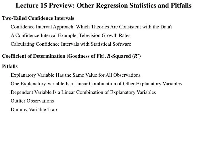
Lecture 15 Preview: Other Regression Statistics and Pitfalls Two-Tailed Confidence Intervals Confidence Interval Approach: Which Theories Are Consistent with the Data? A Confidence Interval Example: Television Growth Rates Calculating Confidence Intervals with Statistical Software Coefficient of Determination (Goodness of Fit), R-Squared (R2) Pitfalls Explanatory Variable Has the Same Value for All Observations One Explanatory Variable Is a Linear Combination of Other Explanatory Variables Dependent Variable Is a Linear Combination of Explanatory Variables Outlier Observations Dummy Variable Trap
Two-Tailed Confidence Intervals Two Approaches to Theory and Data Analysis Our approach thus far has gone from the theory to the data: First, we develop the theory. Second, we analyze the data to determine whether the data are consistent with the theory. The confidence interval approach reverses this process by going from data to theories:. First, we analyze the data. Second, we determine which theories are consistent with the data. Two-Tailed Confidence Intervals and Significance Levels: The “size” of the confidence interval plus its significance level sum to 100 percent. Our Example: 95 percent confidence interval. Significance Level = 5 Percent Confidence Interval Approach: The Conceptual Steps Step 1: Use the ordinary least squares estimation procedure to estimate the models parameters. Step 2: Consider a specific theory. Is the theory consistent with the data? Does the theory lie within the confidence interval? Step 2a: Based on the theory, construct the null and alternative hypotheses. Step 2b: Compute Prob[Results IF H0 True]. The null hypothesis reflects the theory. Step 2c: Do we reject the null hypothesis? Yes: Reject the theory. The data are not consistent with the theory. The theory does not lie within the two-tailed confidence interval. No: The data are consistent with the theory. The theory does lie within the two-tailed confidence interval.
Television Use Growth Rate Confidence Intervals Step 1: Analyze the data. Use the ordinary least squares (OLS) estimation procedure to estimate the model’s parameters. Model: Dependent variable: LogUsersTV Explanatory variables: Year, CapitalHuman, CapitalPhysical, GdpPC, and Auth EViews Step 2:0.0 Percent Growth Rate Theory. Is the 0.0 percent television growth rate theory consistent with the data? Does 0.0 lie within the confidence interval? Step 2a: Based on the theory, construct the null and alternative hypotheses. 0.0 Percent Growth Rate Theory: After accounting for all other explanatory variables, time has no effect on television use; that is, after accounting for all other explanatory variables, the annual growth rate of television use equals 0.0 percent.
Step 2b: Compute Prob[Results IF H0 True]. Prob[Results IF H0 True] = OLS estimation procedure unbiased If H0 were true StandardError Number of observations Number of parameters = .000 = .0159 DF = 742 6 = 736 t-distribution Mean = .000 SE = .0159 Prob[Results IF H0 True] = .1487 DF = 736 .1487/2 .1487/2 Step 2c: Do we reject the null hypothesis? Prob[Results IF H0 True] > .05 .023 .023 .000 .023 Do not reject H0 Question: Can I use the Prob column? Data are consistent with the theory .000 does lie within the 95 percent confidence interval. Question: Yes.
Television Use Confidence Interval Approach Continued – Apply Step 2 Again to a Different Theory Step 2:1.0 Percent Growth Rate Theory. Is the 1.0 percent television growth rate theory consistent with the data? Does 1.0 lie within the confidence interval? Step 2a: Based on the theory, construct the null and alternative hypotheses. 1.0 Percent Growth Rate Theory: After account for all other factors, the annual growth rate of television users is 1.0 percent; that is, Yearequals .010.
Step 2b: Compute Prob[Results IF H0 True]. Prob[Results IF H0 True] = OLS estimation procedure unbiased If H0 were true StandardError Number of observations Number of parameters = .010 = .0159 DF = 742 6 = 736 Right tail probability = .019 Lab 15.2a t-distribution Left tail probability = .019 Mean = .010 SE = .0159 Prob[Results IF H0 True] = .019 + .019 .038 DF = 736 .0191 .0191 Step 2c: Do we reject the null hypothesis? Prob[Results IF H0 True] < .05 .033 .033 .010 .023 Do reject H0 Question: Can I use the Prob column? Data are not consistent with the theory .010 does not lie within the 95 percent confidence interval. Question: No.
Significance Level = 5% = .05 Observations and Two Questions The 0% growth rate theory lies within the 95 percent confidence interval, but 1% theory does not. Question 1: Based on a 5 percent significance level, .05, what is the lowest growth rate theory that is consistent with the data? That is, what is the lower bound of the two-tailed 95 percent confidence interval? The 4% growth rate theory lies within the 95 percent confidence interval, but 6% theory does not. Question 2: Based on a 5 percent significance level, .05, what is the highest growth rate theory that that is consistent with the data? That is, what is the upper bound of the two-tailed 95 percent confidence interval?
Calculating Confidence Intervals with Statistical Software Getting started in EViews: Run the appropriate regression: In the Equation window: Click View, Coefficient Diagnostics, and Confidence Intervals. In the Confidence Intervals window: Enter the confidence levels you wish to compute. (By default the values of .90, .95, and.99 are entered.) Click OK. EViews = .0082 = .0542 At a 95 percent confidence interval, the data are consistent with all the growth rate theories that lie between .82 and 5.42 percent.
Coefficient of Determination (Goodness of Fit) , R-Squared (R2) Theory: Additional studying increases quiz scores. Theory:x > 0 Model:yt =Const + xxt + etxt = Minutes studied yt = Quiz score Hypotheses: H0: x = 0 H1: x > 0 R-squared represents the portion of y’s squared deviations from its mean are explained: Explained Squared Deviations from the Mean 288 = = .84 R2 = = 342 Actual Squared Deviations from the Mean 66 + 87 + 90 Mean of y = = = 81 Claim: R-squared does not assess the “validity” of the theory being assessed. 3 Actual y Actual Explained y Explained Deviation Squared Esty Deviation Squared from Mean Deviation Equals from Mean Deviation Student xtyt 1 5 66 66 81 = 15 225 63 +1.25 = 69 69 81 = 12 144 2 15 87 87 81 = 6 36 63 +1.215 = 81 81 81 = 0 0 3 25 90 90 81 = 9 81 63 +1.225 = 93 93 81 = 12 144 = 342 = 288 Confidence in Theory: Prob[Results IF H0 True] = .2601/2 .13 EViews
Actual y Actual Explained y Explained Deviation Squared Esty Deviation Squared Quiz/ from Mean Deviation Equals from Mean Deviation Student xtyt 1/1 5 66 66 81 = 15 225 63 +1.25 = 69 69 81 = 12 144 1/2 15 87 87 81 = 6 36 63 +1.215 = 81 81 81 = 0 0 1/3 25 90 90 81 = 9 81 63 +1.225 = 93 93 81 = 12 144 2/1 5 66 66 81 = 15 Intuition: Should this increase or decrease your confidence in the theory? 225 63 +1.25 = 69 69 81 = 12 144 2/2 15 87 87 81 = 6 36 63 +1.215 = 81 81 81 = 0 0 Increase. 2/3 25 90 90 81 = 9 81 63 +1.225 = 93 93 81 = 12 144 = 342 684 = 288 576 What about R2? 66 + 87 + 90 66 + 87 + 90 + 66 + 87 + 90 EViews Mean of y = = = 81 6 3 Explained Squared Deviations from the Mean 576 288 = .84 = R2 = = 342 684 Actual Squared Deviations from the Mean Confidence in Theory: Prob[Results IF H0 True] = .0099/2 .005 Does R2 help us assess theories?
Pitfalls Multiple Regression Analysis: Attempts to separate out, to sort out, to isolate the individual influence that each explanatory variable has on the dependent variable. The coefficient estimate of an explanatory variable allows us to estimate by how much the dependent variable changes when that explanatory variable changes while all other explanatory variables remain constant. Dependent variable: Attendance Explanatory variables: PriceTicket and HomeSalary EViews Estimated Equation: EstAttendance = 9,246 – 591PriceTicket + 783HomeSalary
Pitfall: Explanatory Variable Has the Same Value for All Observations Consider the variable DH: DH Dummy variable; 1 if designated hitter permitted; 0 otherwise Our workfile includes only American League games in 1996. Since interleague play did not begin until 1997 and all American League games allow designated hitters, the variable DH will equal 1 for all observations: DH = 1 for all observations EViews This is the software’s way of saying that it cannot perform the calculations that we requested. That is, we as asking the software to do the impossible. Dependent variable: Attendance Explanatory variables: PriceTicket, HomeSalary, and DH The following a warning message appears: Error message: “Near singular matrix.” Intuition: At the most basic level, to determine how an explanatory variable affects the dependent variable, the explanatory variable’s values must vary. Example: Reaction Time Depends on Caffeine Caffeine up Reaction time faster Suggests a relationship Caffeine down Reaction time slower If there is no variation in caffeine consumption, then we cannot observe the effect that the caffeine has on reaction time. More generally, if the is no variation in the explanatory variable, then we cannot observe the effect that the explanatory variable has on the dependent variable. In this case, there is no variation in the DH . Consequently, we cannot observe the effect that DH has on Attendance. In this case, we are asking the software to do the impossible.
Pitfall: One Explanatory Variable Is a Linear Combination of Other Explanatory Variables Review: Include both the ticket price in terms of dollars and the ticket price in terms of cents as explanatory variables: PCents = 100PriceTicket NB: The ticket price in terms of cents was a linear combination of the ticket price in terms of dollars. Dependent variable: Attendance Explanatory variables: PriceTicket, PCents, and HomeSalary This is the software’s way of saying that it cannot perform the calculations that we requested. That is, we are asking the software to do the impossible. EViews The following a warning message appears: Error message: “Near singular matrix.” Review: Multiple regression analysis attempts to separate out, to sort out, to isolate the individual influence that each explanatory variable has on the dependent variable. Intuition: The information contained in PCents is redundant. PCents and PriceTicket contain the same information. The software cannot separate out the individual influence of the two explanatory variables, PriceTicket and PCents, because they contain redundant information.
In fact, any linear combination of explanatory variables produces this problem. EViews To illustrate this consider the following regression: Dependent variable: Attendance Explanatory variables: PriceTicket, HomeSalary, and VisitSalary Now, generate a new variable, TotalSalary: TotalSalary = HomeSalary + VisitSalary NB: TotalSalary is a linear combination of HomeSalary and VisitSalary. Dependent variable: Attendance Explanatory variables: PriceTicket, HomeSalary, VisitSalary, and TotalSalary This is the software’s way of saying that it cannot perform the calculations that we requested. That is, we are asking the software to do the impossible. The following a warning message appears: Error message: “Near singular matrix.” Intuition: The information contained in TotalSalary is redundant. The information contained in TotalSalary is already included in HomeSalary and VisitSalary. The software cannot separate out the individual influence of the three “Salary” explanatory variables because they contain redundant information.
Pitfall: Dependent Variable Is a Linear Combination of Explanatory Variables Dependent variable: TotalSalary Explanatory variables: HomeSalary and VisitSalary EViews The estimates of the coefficients and constant reveal the definition of TotalSalary (the estimate for the constant is effectively 0): TotalSalary = HomeSalary + VisitSalary Furthermore, the standard errors are very small, approximately 0. In fact, they are precisely equal to 0, but they are not reported as 0’s as a consequence of how digital computers process numbers. The regression printout suggests that we are dealing with an “identity,” something that is true by definition.
Pitfall: Outlier Observations EViews Dependent variable: Attendance Explanatory variables: PriceTicket and HomeSalary Home Visiting Home Team Observation Month Day Team Team Salary 1 6 1 Milwaukee Cleveland 20.23200 2 6 1 Oakland New York 19.40450 What is an outlier? An observation that is uniquely different from the others. EViews What if the home team salary were entered incorrectly in the first observation. Home Visiting Home Team Observation Month Day Team Team Salary 1 6 1 Milwaukee Cleveland 20232.00 2 6 1 Oakland New York 19.40450 Even though we changed a single data entry for one nearly six hundred observations, the coefficient estimates of changes dramatically This illustrates how sensitive OLS estimates are to outliers.
Dummy Variable Trap EViews Model 1: Salaryt = Const + SexF1SexF1t + EExperiencet + et SexF1t = 1 if female 0 if male EstSalary = 42,238 2,240SexF1 + 2,447Experience For men: SexF1 = 0 EstSalaryMen = 42,237 0 + 2,447Experience EstSalaryMen = 42,238 + 2,447Experience For women: SexF1 = 1 EstSalaryWomen = 42,237 2,240 + 2,447Experience EstSalaryWomen = 39,998 + 2,447Experience InterceptMen = 42,238 EstSalaryMen = 42,238 + 2,447Experience Salary InterceptWomen = 39,998 Slope = 2,447 Question: How many parameter estimates did we use to estimate the value of the 2 intercepts? 2 bConst and bSexF1 42,238 2,240 Dummy Variable Trap: A model in which there are more parameters representing the intercepts than there are intercepts. EstSalaryWomen = 39,998 + 2,447Experience 39,998 Experience
Model 2: Salaryt = Const + SexM1SexM1t + EExperiencet + et SexM1t = 1 if male 0 if female EstSalary = bConst + bSexM1SexM1 + bEExperience Question: Can we determine the values of bConst and bSexM1in this model from the intercepts we calculated from Model 1? InterceptMen = 42,238 InterceptWomen = 39,998 For men For women SexM1 = 1 SexM1 = 0 EstSalaryMen = bConst + bSexM1 + bEExperience EstSalaryWomen = bConst + bEExperience InterceptMen = bConst + bSexM1 InterceptWomen = bConst 42,238 = bConst + bSexM1 39,998 = bConst Unknowns = 2 Equations = 2 Can we solve for the two unknowns? Yes bConst = 39,998 bSexM1 = 42,238 bConst = 42,238 39,998 = 2,240 EViews
Model 3: Salaryt = SexM1SexM1t + SexF1SexF1t + EExperiencet + et EstSalary = bSexM1SexM1 + bSexF1SexF1 + bEExperience Question: Can we determine the values of bSexM1and bSexF1 in this model from the intercepts we calculated from Model 1? InterceptMen = 42,238 InterceptWomen = 39,998 For men For women SexM1=1 and SexF1 = 0 SexM1 = 0 and SexF1 = 1 EstSalaryMen = bSexM1 + bEExperience EstSalaryWomen = bSexF1 + bEExperience InterceptMen = bSexM1 InterceptWomen = bSexF1 42,238 = bSexM1 39,998 = bSexF1 Unknowns = 2 Equations = 2 Can we solve for the unknowns? Yes bSexM1 = 42,238 bSexF1 = 39,998 EViews
Model 4: Salaryt = Const+ SexM1SexM1t + SexF1SexF1t + EExperiencet + et EstSalary = bConst + bSexM1SexM1 + bSexF1SexF1 + bEExperience Question: Can we determine the values of bConst, bSexM1, and bSexF1in this model from the intercepts we calculated from Model 1? InterceptMen = 42,238 InterceptWomen = 39,998 For men For women SexM1=1 and SexF1 = 0 SexM1 = 0 and SexF1 = 1 EstSalaryMen = bConst + bSexM1+ bEExperience EstSalaryWomen = bConst + bSexF1 + bEExperience InterceptMen = bConst + bSexM1 InterceptWomen = bConst + bSexF1 42,238 = bConst + bSexM1 39,998 = bConst + bSexF1 Unknowns = 3 Equations = 2 Can we solve for the three unknowns? No bConst When we try to run this regression we are asking the software to do the impossible. bSexM1 EViews bSexF1 That is why we get the “Near singular matrix” error message. Dummy Variable Trap: A model in which there are more parameters representing the intercepts than there are intercepts.