Download

1 / 26
260 likes | 396 Vues
Historical Perspective on Forest Area Estimation (SRS). Raymond M. Sheffield. In the Beginning…. Southeast South Central SRS ~ 1960’s to 2005. Southeast—historical overview. 1933-1940

E N D
Historical Perspective on Forest Area Estimation (SRS) Raymond M. Sheffield
In the Beginning…. • Southeast • South Central • SRS • ~ 1960’s to 2005
Southeast—historical overview • 1933-1940 • Forest/nonforest determined from classification of land use at ground sample plots (strips 10 mi apart-plots at 660 ft. intervals) • 1946-1957 • Photography based • Dot grid overlay (1 acre circles classified) • Forest estimates based on proportion of total points classed as forest • Adjusted based on ground samples • Forest / nonforest samples not proportional to land use
Southeast—historical overview • 1957-1968 • Basically same as 1946-1957 except for numerous changes in land use classes identified • 1968 • 16-point cluster double sample design
16-point Cluster Double Sample Design • Photo based • Estimation unit: County • County land area (or total area) obtained from Bureau of Census • Cluster of points rather than single points • Forest/nonforest proportion of each cluster treated as a continuous variable • Unadjusted forest proportion based on forest points / total points • Double sample design • Subsample of the clusters are ground checked
16-point Cluster Double Sample Design • Linear regression fitted to develop photo/ground relationship • Adjusted proportion of forest developed from regression
16-point cluster--logistics • Photos acquired for approx. 100% coverage of county • 25 16-point clusters per photograph • 16 point clusters stamped on each ground plot (subsample) • Average area/point classified ranged from 12 to 20 acres
An Example • Mitchell County, GA • Total land area: 327,699 acres • 16-point clusters: 1,473 • Total points: 23,568 • Forest points: 8,350 • Ground plots: 113
An Example • Unadjusted forest proportion (P) • P = # Forest points/Total points • P = 8,350/23,568 • P = 0.354294
Adjusted Forest Proportion (AP) • AP = a + b (P) • AP = 0.018479 + .994552 (.354294) • AP = 0.370843
Notes • Intensive sample of photo points and ground plots • Labor intensive • Ground plots randomly distributed….not on a systematic grid
South Central—historical overview • Not much detail available describing forest area procedures in first inventories • In 1960’s, a grid of points overlaid on photos was standard with a subsample of ground plots—Point Based Double Sample Design
Point-based Double Sample Design • Photo based • Estimation unit: County • County land area (or total area) obtained from Bureau of Census • Single points classed as forest or nonforest. Grid of 25 points placed over photos—one photo per ground plot (plots on a 3 x 3 mi. grid) • Unadjusted forest proportion based on forest points / total points
Point-based Double Sample Design • Forest / nonforest classifications made for each ground plot • The photo vs ground classification is used to “correct” the initial forest proportion • Ground correction strengthened by using intensification plots (only photo and ground check of land use) • Average area/point classified approx. 228 acres
An Example • See handout • AP = ((# forest dots)(CF1) + (# nonforest dots)(CF2)) / Total dot count • CF1 = (# plots correctly PI’d forest) / (Total number plots PI’d forest) • CF2 = (# plots PI’d nonforest but actually forest) / (total plots PI’d nonforest) • AP = ((1962 x .973) + (1288 x .0241)) / 3250 • AP = .5969
Photo’s F NF 2 F 108 110 3 81 84 NF 111 83 194 Current Method of Area Correction (# Forest PI’s x CF1) + (# Nonforest PI’s x CF2) Total PI’s (1962 x .973) + (1288 x .024) 3250 .5969 Forest area = .5969 x census land % Forest = = = Plots
Merged SRS-FIA • Continued use of 25 point double sampling design • Used from 1998-2004 • Converted to a 27x intensification of 6000 acre hex
Ground plot sampled by field crews The nested P1 grid
Ray’s Observations • 25 point double sampling design would probably have performed better using the survey unit as the estimation unit • Correction factors were often quite large for single counties • Small counties • Different classifiers at each phase of the double sample • Implementing in annual inventory mode had many rough spots • Changing plot list • Out dated photography • 25 point grid often overlapped with adjoining plot and photo
Ray’s Observations • Photo based systems consume people • Often utilize inexperienced observers for photo classification