
Chapter 10: Linear Regression
E N D
Presentation Transcript
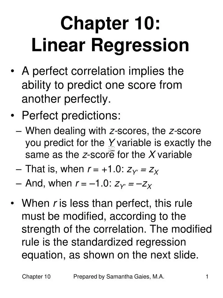
Chapter 10: Linear Regression • A perfect correlation implies the ability to predict one score from another perfectly. • Perfect predictions: • When dealing with z-scores, the z-score you predict for the Y variable is exactly the same as the z-score for the X variable • That is, when r = +1.0: zY’= zX • And, when r = –1.0: zY’ = –zX • When r is less than perfect, this rule must be modified, according to the strength of the correlation. The modified rule is the standardized regression equation, as shown on the next slide. Prepared by Samantha Gaies, M.A.
Predicting with z-scores • Standardized Regression Equation: zY’ = r zX • If r = –1 or +1, the magnitude of the predicted z score is the same as the z score from which we are predicting. • If r = 0, the z score prediction is always zero (i.e., the mean), which implies that, given no other information, our best prediction for a variable is its own mean. • As the magnitude of r becomes smaller, there is less of a tendency to expect an extreme score on one variable to be associated with an equally extreme score on the other. This is consistent with Galton’s concept of “regression toward mediocrity” (i.e., regression toward the mean). Prepared by Samantha Gaies, M.A.
Raw score graph z score graph Prepared by Samantha Gaies, M.A.
Regression Formulas when Dealing with a Population • A basic formula for linear regression in terms of population means and standard deviations is as follows: • This formula can be simplified to the basic equation for a straight line: where and Prepared by Samantha Gaies, M.A.
Regression Formulas for Making Predictions from Samples • The same raw-score regression equa-tion is used when working with samples: except that the slope of the line is now found from the unbiased SDs: and the Y-intercept is now expressed in terms of the sample means: Prepared by Samantha Gaies, M.A.
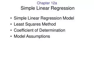
Quantifying the Errors around the Regression Line • Residual:the difference between the actual Y value and the predicted Yvalue (Y – Y’). Each residual can be thought of as an error of prediction. • The positive and negative residuals will balance out so that the sum of the residuals will always be zero. • The linear regression equation gives us the straight line that minimizes the sum of the squared residuals (i.e., the sum of squared errors). Therefore, it is called the least-squares regression line. • The regression line functions like a running average of Y, in that it passes through the mean of the Y values (approximately) for each value of X. Prepared by Samantha Gaies, M.A.
The Variance of theEstimate in a Population • Quantifies the average amount of squared error in the predictions: • The variance of the estimate (or residual variance) is the variance of the data points around the regression line. • As long as r is not zero, σ2estYwill be less than σ2Y (the ordinary variance of the Y values); the amount by which it is less represents the advantage of performing regression. • Larger rs (in absolute value) will lead to less error in prediction (i.e., points closer to the regression line) and therefore a smaller value for σ2estY. • This relation between σ2estY and Pearson’s r is shown in the following formula: Prepared by Samantha Gaies, M.A.
Coefficient of Determination • The proportion of variance in the predicted variable that isnotaccounted for by the predicting variable is found by rearranging the formula for the variance of the estimate in the previous slide. 1 – r 2 = unexplained variance = σ2estY total variance σ2Y • The ratio of the variance of the estimate to the ordinary variance of Y is called the coefficient of nondetermination, and it is sometimes symbolized as k2. • Larger absolute values of r are associated with smaller values for k2. • The proportion of the total variance that is explained by the predictor variable is called the coefficient of determination, and it is simply equal to r2: r 2 = explained variance = 1 – k2 total variance Prepared by Samantha Gaies, M.A.
Here is a concrete example of Linear Regression … Example from Lockhart, Robert S. (1998). Introduction to Statistics and Data Analysis. New York: W. H. Freeman & Company. Prepared by Samantha Gaies, M.A.
Estimating the Variance of the Estimate from a Sample • When using a sample to estimate the variance of the estimate, we need to correct for bias, even though we are basing our formula on the unbiased estimate of the ordinary variance: Standard Error of the Estimate The standard error of the estimate is just the square root of the variance of the estimate. When estimating from a sample, the formula is: Prepared by Samantha Gaies, M.A.
Assumptions Underlying Linear Regression • Independent random sampling • Bivariate normal distribution • Linearity of the relationship between the two variables • Homoscedasticity (i.e., the variance around the regression line is the same for every X value) Uses for Linear Regression • Prediction • Statistical control (i.e., removing the linear effect of one variable on another) • Quantifying the relationship between a DV and a manipulated IV with quantita-tive levels. Prepared by Samantha Gaies, M.A.
The Point-Biserial Correlation Coefficient • An ordinary Pearson’s r calculated for one continuous multivalued variable and one dichotomous (i.e., grouping) variable. The sign of rpb is arbitrary and therefore usually ignored. • A rpb can be tested for significance with a one-sample t test as follows: • By solving for rpb, we obtain a simple formula for converting a two-sample pooled-variance t value into a corre-lational measure of effect size: Prepared by Samantha Gaies, M.A.
The Proportion of Variance Accounted for in a Two-Sample Comparison • Squaring rpb gives the proportion of vari-ance in your DV accounted for by your two-level IV (i.e., group membership). • Even when you obtain a large t value, it is possible that little variance is accounted for; therefore, rpb is a useful supplement to the two-sample t value. • rpb is an alternative to g for expressing the effect size found in your samples. The two measures have a fairly simple relationship: where N is the total number of cases across both groups, and df = N – 2 Prepared by Samantha Gaies, M.A.
Estimating the Proportion of Variance Accounted for in the Population • r2pb from a sample tends to over-estimate the proportion of variance accounted for in the population. This bias can be corrected with the following formula: • ω2 and d 2 are two different measures of the effect size in the population. They have a very simple relationship, as shown by the following formula: Prepared by Samantha Gaies, M.A.