The Binary Genetic Algorithm
The Binary Genetic Algorithm. Universidad de los Andes-CODENSA. 1. Genetic Algorithms: Natural Selection on a Computer.

The Binary Genetic Algorithm
E N D
Presentation Transcript
The Binary Genetic Algorithm Universidad de los Andes-CODENSA
1. Genetic Algorithms: Natural Selection on a Computer Figure 1 shows the analogy between biological evolution and a binary GA. Both start with an initial population of random members. Each row of binary numbers represents selected characteristics of one of the dogs in they population. Traits associated with loud barking are encoded in the binary sequence associated with these dogs.
Figure 1. Analogy between a numerical GA and biological genetics.
2. Components of a Binary Genetic Algorithm The GA begins, like any other optimization algorithm, by defining the optimization variables, the cost function, and the cost. It ends like other optimization algorithms too, by testing for convergence. In between, however, this algorithm is quite different. A path through the components of the GA is shown as a flowchart in Figure 2. The cost function is like a surface with peaks and valleys when displayed in variable space, much like a topographic map. To find a valley. An optimization algorithm searches for the minimum cost. To find a peak, an optimization algorithm searches for the maximum cost. Figures 3 and 4 show examples of 3D plot of a portion of the park and a crude topographical map, respectively. Since there are many peaks in the area of interest, conventional optimization techniques have difficulty finding Long’s peak unless the starting point is in the immediate vicinity of the peak. In fact all the methods requiring a gradient of the cost function won’t work well with discrete data. The GA has no a problem.
Figure 3. Three dimensional view of the cost surface with a view of Long’s Peak. Figure 4. Topographical map of the cost surface around Long’s Peak.
2.1. Selecting the Variables and the Cost Function A cost function generates an output from a set of input variables (a chromosome). The cost function may be a mathematical function, an experiment, or a game. The object is to modify the output in some desirable fashion by finding the appropriate values for the input variables. The GA begins by defining a chromosome or an array of variable values to be optimized. If the chromosome has Nvar variables (an Nvar -dimensional optimization problem) given by p1, p1,…, pNvar , the chromosome is written as an Nvar element row vector. Each chromosome has a cost found by evaluating the cost function , f, at p1, p2,…,pNvar.
Often the cost function is quite complicated, as in maximizing the gas mileage of a car. The user must decide which variables of the problem are more important. Too many variables bog down the GA. Important variables for optimizing the gas mileage might include size of the car, size of the engine, and weight of the materials. Other variables, such as paint color and type of headlights, have little or no impact on the car gas mileage and should not be included. Sometimes the correct number and choice of variables comes from experience or trial optimization runs. Other times we have an analytical cost function. Most optimization problems require constraints or variable bounds. Unconstrained variables can take any value. Constrained variables come in three brands: • Hard limits in the form of >, <, ≥ and ≤ can be imposed on the variables. When a variable exceeds a bound, then it is set equal to that bound. • Variables can be transformed into new variables that inherently include the constraints. • There may be a finite set of variable values from which to choose, and values lie within the region of interest.
Dependent variables present special problems for optimization algorithms because varying one variable also changes the value of the other variable. Independent variables, like Fourier series coefficients, do not interact with each other. In the GA literature, variable interaction is called epistasis (a biological term for gene interaction). When there is little to no epistasis, minimum seeking algorithm perform best. Gas shine when epistasis is medium to high, and pure random search algorithms are champions when epistasis is very high, like figure 5. Figure 5. Epistasis Thermometer.
2.2. Variable Encoding and Decoding Since the variable values are presented in binary, there must be a way of converting continues values into binary, and visa versa. Quantization samples a continues range of values and categorizes the samples into nonoverlapping subranges. Then a unique discrete value is assigned to each subrange. The difference between the actual function value and the quantization level is known as the quantization error. Figure 6. A Bessel function and 6-bit quantized version of the same function.
Quantization begins by sampling a function and placing the samples into equal quantization levels (Figure 7). Figure 7. Four continues parameters values are graphed with the quantization levels shown. The corresponding gene or chromosome indicates the quantization level where the parameter value falls.
The mathematical formulas for the binary encoding and decoding of the nth variable, pn, are given as follows: For encoding, For decoding, In each case pnorm: normalized variable, 0 ≤ pnorm ≤ 1 plo: smallest variable value phi: highest variable value Gen[m]: binary version of pn
Round{.}: round to nearest integer Pquant: quantized version of pnorm qn: quantized version of pn The binary GA works with bits. Table 1. Decoding a gene. Table 2. Binary representations.
The quantized value of the gene or variable is mathematically found by multiplying the vector containing the bits by a vector containing the quantization levels: where: gene: [b1 b2… bNgene] Ngene: number bits in a gene bn: binary bit (1 or 0) Q: quantization vector [2-1 2-2 … 2Ngene] QT: transpose of Q The GA works with the binary encodings, but the cost function often requires continues variables. Whenever the cost function is evaluated, the chromosome must first be decoding. An example of a binary encoded chromosome (Ngene=10 bits)is:
2.3. The Population The GA starts with a group of chromosomes known as the population. The population has Npopchromosomes and is an Npop x Nbits matrix filled with random ones and zeros generated using where the function (Npop, Nbits) generates a Npop x Nbits matrix of uniform random numbers between zero and one. Table 3. Example initial population of 8 random chromosomes and their corresponding cost.
Figure 8. A contour map of the cost surface with the 8 initial population members indicated by large dots.
2.4. Natural Selection Survival of the fittest translates into discarding the chromosomes with the highest cost (Figure 9). First, the Npop costs and associated chromosomes are ranked from lowest cost to highest cost. Then, only the best are selected to continue, while the rest are deleted. The selection rate, xrate, is the fraction of Npop that survives for the next step of mating. The number of chromosomes that are kept each generation is Natural selection occurs each generation or iteration of the algorithm. Of the Npop chromosomes in a generation, only the top Nkeep survive for mating, and the bottom Npop – Nkeep are discarded to make room for the new offspring. Deciding how many chromosomes to keep is somewhat arbitrary. Letting only a few chromosomes survive to the next generation limits the available genes in the offspring. Keeping too many chromosomes allows bad performers a chance to contribute their traits to the next generation. It is common 50% (xrate=0.5) in the natural selection process.
In our example, Npop =8. With a 50% selection rate, Nkeep=4. The natural selection results are shown in table 4. Then the four with the lowest cost survive to the next generation and become potential parents. Figure 9. Individuals with the best traits survive. Unfit species in nature don’t survive. Table 4. Surviving Chromosomes after 50% selection rate.
Another approach to natural selection is called thresholding. In this approach all chromosomes that have a cost lower than some threshold survive. The threshold must allow some chromosomes to continue in order to have parents to produce offspring. Otherwise, a whole new population must be generated to find some chromosomes that pass the test. At first, only a few chromosomes may survive. In later generations, however, most of the chromosomes will survive unless the threshold is changed. An attractive feature of this technique is that the population does not have to be sorted.
2.5. Selection Two chromosomes are selected from the mating pool of Nkeep chromosomes to produce two new offspring. Pairing takes place in the mating population until Npop-Nkeep offspring are born to replace the discarded chromosomes. Pairing chromosomes in a GA can be as interesting and varied as in animal species. The selection methods are: • Pairing from top to bottom. Start at the top of the list and pair the chromosomes two at a time until the top Nkeep chromosomes are selected for mating. Thus, the algorithm pairs odd rows with even rows. The mother has row numbers in the population matrix given by ma=1,3,5,… and father has the row numbers pa=2,4,6,… This approach doesn’t model nature well but is very simple to program.
Random Pairing. This approach uses a uniform random number generator to select chromosomes. The row numbers of the parents are found using where ceil rounds the value to the next highest integer. • Weighted random pairing. The probabilities assigned to the chromosomes in the mating pool are inversely proportional to their cost. A chromosome with the lowest cost has the greatest probability of mating, while the chromosome with the highest cost has the lowest probability of mating. A random number determines which chromosome is selected. This type of weighting is often referred to as roulette wheel weighting. There are two techniques: • Rank weighting • Cost weighting
Rank weighting. This approach is problem independent and finds the probability from the rank, n, of the chromosome: Table 5 shows the results for the Nkeep=4 chromosomes. Table 5. Rank weighting.
Cost weighting. The probability of selection is calculated from the cost of the chromosome rather than its rank in the population. A normalized cost is calculated for each chromosome by subtracting the lowest cost of the discarded chromosomes (cNkeep+1) from the cost of all the chromosomes in the mating pool: Subtracting cNkeep+1 ensures all the costs are negative. Table 6 lists the normalized costs assuming that cNkeep+1=-12097. Pn is calculated from: This approach tends to weight the top chromosome more when there is a large spread in the cost between the top and bottom chromosome. On the other hand, it tends to weight the chromosomes evenly when all the chromosomes have approximately the same cost. The same issues apply if a chromosome is selected to mate with itself. The probabilities must be recalculated each generation.
Table 6. Cost weighting. • Tournament selection. Another approach that closely mimics mating competition in nature is randomly pick a small subset of chromosomes (two or three) from the mating pool, and the chromosome with the lowest cost in this subset becomes a parent. The tournament repeats for every parent needed. Thresholding an tournament selection make a nice pair, because the population never needs to be sorted. Figure 10 shows the probability of selection for five selection methods.
Figure 10. Graph of the probability of selection for 8 parents using five different methods of selection.
2.6. Mating Mating is the creation of one or more offspring from the parents selected in the pairing process. The genetic makeup of the population is limited by the current members of the population. The most common form of mating involves two parents that produce two offspring (figure 11). A cross over point, or kinetochore, is randomly selected between the first and the last bits of the parent’s chromosomes. Figure 11. Two parents mate to produce two offspring. The offspring are placed into the population.
Table 7 shows the pairing and mating process for the problem at hand. Table 7. Pairing and mating process of single-point crossover.
2.7. Mutations Random mutations alter a certain percentage of the bits in the list of chromosomes. Mutation is the second way a GA explores a cost surface. It can introduce traits not in the original population and keeps the GA from converging too fast before sampling the entire cost surface. A single point mutation changes a 1 to a 0, and visa versa. Mutation point are randomly selected from the Npop x Nbits total number of bits in the population matrix. Increasing the number of mutations increases the algorithm’s freedom to search outside the current region of variable space. It also tends to distract the algorithm form converging on a popular solution. The number of mutations is given by
The computer code to find the rows and columns of the mutated bits is Locations of the chromosomes at the end of the first generation are shown in figure 12. Table 8. Mutating the population.
Figure 12. A contour map of the cost surface with the 8 members at the end of the first generation.
2.8. The Next generation After the mutations take place, the costs associated with the offspring and mutated chromosomes are calculated. The process described is iterated. After mating, mutation and ranking, the population is shown in table 12 and figure 14. Table 9. New rank population at the start of the second generation.
Table 10. Population after crossover and mutation in the second generation. Figure 13. A contour map of the cost surface with the 8 members at the end of the second generation.
Table 11. New ranked population at the start of the third generation. Table 12. Ranking of generation 2 from least to most cost.
Figure 14. A contour map of the cost surface with the 8 members at the end of the third generation.
2.9. Convergence The number of generations that evolve depends on whether an acceptable solution is reached or a set number of iterations is exceeded. After a while all the chromosomes and associated costs would become the same if it were not for mutations. At this point the algorithm should be stopped. Most GAs keep track of the population statistics in the form of population mean and minimum cost. Figure 15 shows a plot of the algorithm convergence in terms of the minimum and mean cost of each generation. Figure 15. Graph of the of the mean cost and minimum cost for each generation.
3. Program in MATLAB N=200; % number of bits in a chromosome M=8; % number of chromosomes must be even last=50; % number of generations sel=0.5; % selection rate M2=2*ceil(sel*M/2); % number of chromosomes kept mutrate=0.01; % mutation rate nmuts=mutrate*N*(M-1); % number of mutations % creates M random chromosomes with N bits pop=round(rand(M,N)); % initial population for ib=1:last cost=costfunction(pop); % cost function % ranks results and chromosomes [cost,ind]=sort(cost); pop=pop(ind(1:M2),:); [ib cost(1)]
% mate cross=ceil((N-1)*rand(M2,1)); % pairs chromosome and performs crossover for ic=1:2:M2 pop(ceil(M2*rand),1:cross)=pop(ic,1:cross); pop(ceil(M2*rand),cross+1:N)=pop(ic+1,cross+1:N); pop(ceil(M2*rand),1:cross)=pop(ic+1,1:cross); pop(ceil(M2*rand),cross+1:N)=pop(ic,cross+1:N); end % mutate for ic=1:nmuts ix=ceil(M*rand); iy=ceil(N*rand); pop(ix,iy)=1-pop(ix,iy); end % ic end % ib
4. Bibliography • Randy L. Haupt and Sue Ellen Haupt. “Practical Genetic Algorithms”. Second edition. 2004.