Automatic control theory
Automatic control theory. A Course ——used for analyzing and designing a automatic control system. * Operating principle……. * Feedback control……. Figure 1.1. Chapter 1 Introduction.

Automatic control theory
E N D
Presentation Transcript
Automatic control theory A Course ——used for analyzing and designing a automatic control system
* Operating principle…… * Feedback control…… Figure 1.1 Chapter 1 Introduction 21 century — information age, cybernetics(control theory), system approach and information theory , three science theory mainstay(supports) in 21 century. 1.1 Automatic control A machine(or system) work by machine-self, not by manual operation. 1.2 Automatic control systems 1.2.1 examples 1) A water-level control system
* Operating principle…… * Feedback control…… * Operating principle… * Feedback control(error)… Chapter 1 Introduction Another example of the water-level control is shown in figure 1.2. 2) A temperature Control system (shown in Fig.1.3)
* Principle… * Feedback control(error)… Chapter 1 Introduction 3) A DC-Motor control system
* principle…… * feedback(error)…… Chapter 1 Introduction 4) A servo (following) control system Fig. 1.5
* principle…… * feedback(error)…… Chapter 1 Introduction 5) A feedback control system model of the family planning (similar to the social, economic, and political realm(sphere or field)) Fig. 1.6
Chapter 1 Introduction 1.2.2 block diagram of control systems The block diagram description for a control system :Convenience Fig. 1.7 Example:
resistance comparator Actual Desired water level water level Water amplifier Motor Gearing Valve container Input Output Float Figure 1.1 Chapter 1 Introduction For the Fig.1.1, The water level control system: Actuator Error Process controller Feedback signal measurement (Sensor) Fig. 1.8
Chapter 1 Introduction For the Fig. 1.4, The DC-Motor control system
Chapter 1 Introduction 1.2.3 Fundamental structure of control systems 1) Open loop control systems Features: Only there is a forward action from the input to the output.
Features: not only there is a forward action , also a backward action between the output and the input (measuring the output and comparing it with the input). 1) measuring the output (controlled variable) . 2) Feedback. Chapter 1 Introduction 2) Closed loop (feedback) control systems
Chapter 1 Introduction Notes:1) Positive feedback; 2) Negative feedback—Feedback. 1.3 types of control systems 1) linear systems versus Nonlinear systems. 2) Time-invariant systems vs. Time-varying systems. 3) Continuous systems vs. Discrete (data) systems. 4) Constant input modulation vs. Servo control systems. 1.4Basic performance requirements of control systems 1) Stability. 2) Accuracy (steady state performance). 3) Rapidness (instantaneous characteristic).
Chapter 1 Introduction 1.5 An outline of this text 1) Three parts:mathematical modeling; performance analysis ; compensation (design). 2) Three types of systems: linear continuous; nonlinear continuous; linear discrete. 3) three performances:stability, accuracy, rapidness. in all: to discuss the theoretical approaches of the control system analysis and design. 1.6 Control system design process shown in Fig.1.12
1. Establish control goals 6.Describe a controller and select key parameters to be adjusted 2. Identify the variables to control 7. Optimize the parameters and analyze the performance 3. Write the specifications for the variables Performance meet the specifications Performance does not Meet the specifications 4. Establish the system configuration Identify the actuator Finalize the design 5.Obtain a model of the process, the actuator and the sensor Fig.1.12 Chapter 1 Introduction
Rotation of arm Spindle Track a Disk Track b Actuator motor Arm Head slider Fig.1.13 A disk drive read system Chapter 1 Introduction A disk drive read system Shown in Fig.1.13 1.7 Sequential design example: disk drive read system ◆Configuration ◆ Principle
Chapter 1 Introduction Sequential design: here we are concerned with the design steps 1,2,3, and 4 of Fig.1.12. • Identify the control goal: Position the reader head to read the date stored on a track on the disk. (2) Identify the variables to control: the position of the read head. (3) Write the initial specification for the variables: The disk rotates at a speed of between 1800 and 7200 rpm and the read head “flies” above the disk at a distance of less than 100 nm. The initial specification for the position accuracy to be controlled: ≤ 1 μm (leas than 1 μm ) and to be able to move the head from track a to track b within 50 ms, if possible.
Desired head position Actual head position error Control device Actuator motor Read arm sensor Fig.1.13 system configuration for disk drive Chapter 1 Introduction It is obvious : we should propose a closed loop system , not a open loop system. (4) Establish an initial system configuration: An initial system configuration can be shown as in Fig.1.13. We will consider the design of the disk drive further in the after-mentioned chapters.
Chapter 1 Introduction Exercise: E1.6, P1.3, P1.13
Disturbance e(t)= u u + r(t)-b(t) Output T(t) Input r(t) k a c Controller Actuator Process actual output temperature - desired output temperature Control Actuating (-) signal signal Feedback signal b(t) temperature measurement Fig. 2.1 Chapter 2 mathematical models of systems 2.1.1 Why? 1) Easy to discuss the full possible types of the control systems—in terms of the system’s “mathematical characteristics”. 2) The basis — analyzing or designing the control systems. For example, we design a temperature Control system : 2.1 Introduction The key — designing the controller → how produce uk.
T(t) For T1 T2 T1 uk For T1 uk11 uk12 uk21 Chapter 2 mathematical models of systems Different characteristic of the process — differentuk: Ⅰ Ⅱ 2.1.2 What is ? Mathematical models of the control systems—— the mathematical relationships between the system’s variables. 2.1.3 How get? 1) theoretical approaches 2) experimental approaches 3) discrimination learning
Chapter 2 mathematical models of systems 2.1.4 types 1) Differential equations 2) Transfer function 3) Block diagram、signal flow graph 4) State variables(modern control theory) 2.2 Input-output description of the physical systems — differential equations The input-output description—description of the mathematical relationship between the output variable and the input variable of the physical systems. 2.2.1 Examples
Chapter 2 mathematical models of systems Example 2.1 : A passive circuit define: input → ur output → uc。 we have:
Chapter 2 mathematical models of systems Define: input → F ,output → y. We have: Example 2.2 : A mechanism Compare with example 2.1: uc→y; ur→F ─ analogous systems
Chapter 2 mathematical models of systems Input →ur output →uc Example 2.3 : An operational amplifier (Op-amp) circuit (2)→(3); (2)→(1); (3)→(1):
Chapter 2 mathematical models of systems Example 2.4 : A DC motor Input → ua, output → ω1 (4)→(2)→(1) and (3)→(1):
Chapter 2 mathematical models of systems The differential equation description of the DC motor is: Assume the motor idle: Mf = 0, and neglect the friction: f = 0, we have:
Chapter 2 mathematical models of systems Example 2.5 : A DC-Motor control system Input → ur,Output → ω; neglect the friction:
Chapter 2 mathematical models of systems (2)→(1)→(3)→(4),we have: 2.2.2 steps to obtain the input-output description (differential equation) of control systems 1) Determine the output and input variables of the control systems. 2) Write the differential equations of each system’s components in terms of the physical laws of the components. * necessary assumption and neglect. * proper approximation.
Chapter 2 mathematical models of systems 3) dispel the intermediate(across) variables to get the input-output description which only contains the output and input variables. 2.2.3 General form of the input-output equation of the linear control systems—A nth-order differential equation: 4) Formalize the input-output equation to be the “standard” form: Input variable —— on the right of the input-output equation . Output variable —— on the left of the input-output equation. Writing polynomial—— according to the falling-power order. Suppose:input → r ,output → y
Chapter 2 mathematical models of systems 2.3 Linearization of the nonlinear components 2.3.1 what is nonlinearity? The output is not linearly vary with the linear variation of the system’s (or component’s) input → nonlinear systems (or components). 2.3.2 How do the linearization? Suppose: y = f(r) The Taylor series expansion about the operating point r0 is:
Chapter 2 mathematical models of systems Example 2.6 : Elasticity equation Examples: Example 2.7 : Fluxograph equation Q —— Flux; p —— pressure difference
Chapter 2 mathematical models of systems 2.4 Transfer function Another form of the input-output(external) description of control systems, different from the differential equations. 2.4.1 definition Transfer function:The ratio of the Laplace transform of the output variable to the Laplace transform of the input variable,with all initial condition assumed to be zero and for the linear systems,that is:
Chapter 2 mathematical models of systems C(s) —— Laplace transform of the output variable R(s) —— Laplace transform of the input variable G(s) —— transfer function Notes: * Only for the linear and stationary(constant parameter) systems. * Zero initial conditions. * Dependent on the configuration and the coefficients of the systems, independent on the input and output variables. 2.4.2 How to obtain the transfer function of a system 1) If the impulse response g(t) is known
Chapter 2 mathematical models of systems We have: Because: Then: Example 2.8 : 2) If the output response c(t) and the input r(t) are known We have:
Chapter 2 mathematical models of systems Example 2.9: Then: 3) If the input-output differential equation is known • Assume: zero initial conditions; • Make: Laplace transform of the differential equation; • Deduce: G(s)=C(s)/R(s).
Chapter 2 mathematical models of systems Example 2.10: 4) For a circuit * Transform a circuit into a operator circuit. *Deduce the C(s)/R(s) in terms of thecircuits theory.
Chapter 2 mathematical models of systems Example 2.11: For a electric circuit:
Chapter 2 mathematical models of systems Example 2.12: For a op-amp circuit
Chapter 2 mathematical models of systems • Write the differential equations of the control system, and Assume zero initial conditions; • Make Laplace transformation, transform the differential equations into the relevant algebraic equations; • Deduce: G(s)=C(s)/R(s). 5) For a control system Example 2.13 the DC-Motor control system in Example 2.5
Chapter 2 mathematical models of systems In Example 2.5, we have written down the differential equations as: Make Laplace transformation, we have:
Chapter 2 mathematical models of systems (2)→(1)→(3)→(4), we have:
Chapter 2 mathematical models of systems 2.5 Transfer function of the typical elements of linear systems A linear system can be regarded as the composing of several typical elements, which are: 2.5.1 Proportioning element Relationship between the input and output variables: Transfer function: Block diagram representation and unit step response: Examples: amplifier, gear train, tachometer…
Chapter 2 mathematical models of systems Relationship between the input and output variables: 2.5.2 Integrating element Transfer function: Block diagram representation and unit step response: Examples: Integrating circuit, integrating motor, integrating wheel…
Chapter 2 mathematical models of systems Relationship between the input and output variables: 2.5.3 Differentiating element Transfer function: Block diagram representation and unit step response: Examples: differentiating amplifier, differential valve, differential condenser…
Chapter 2 mathematical models of systems Relationship between the input and output variables: 2.5.4 Inertial element Transfer function: Block diagram representation and unit step response: Examples: inertia wheel, inertial load (such as temperature system)…
Chapter 2 mathematical models of systems Relationship between the input and output variables: 2.5.5 Oscillating element Transfer function: Block diagram representation and unit step response: Examples: oscillator, oscillating table, oscillating circuit…
Chapter 2 mathematical models of systems Relationship between the input and output variables: 2.5.6 Delay element Transfer function: Block diagram representation and unit step response: Examples: gap effect of gear mechanism, threshold voltage of transistors…
Chapter 2 mathematical models of systems 2.6 block diagram models (dynamic) Portray the control systems by the block diagram models more intuitively than the transfer function or differential equation models. 2.6.1 Block diagram representation of the control systems Examples:
Chapter 2 mathematical models of systems For the DC motor in Example 2.4 In Example 2.4, we have written down the differential equations as: Example 2.14 Make Laplace transformation, we have: