Automatic Control System
Automatic Control System. II. Block diagram model. Modelling dynamical systems. Engineers use models which are based upon mathematical relationships between two variables . We can define the mathematical equations : Measuring the responses of the built process (b lack model )

Automatic Control System
E N D
Presentation Transcript
Automatic ControlSystem II. Block diagram model
Modelling dynamical systems • Engineers use models which are based upon mathematical relationships between two variables. • We can define the mathematical equations: • Measuring the responses of the built process (black model) • Using the basic physical principles (greymodel). In order to simplification of mathematical model the small effects are neglected and idealised relationships are assumed. • Developing a new technology or a new construction nowadays it’s very helpful applying computer aided simulation technique. • This technique is very cost effective, because one can create a model from the physical principles without building of process.
LTI (Linear Time Invariant) model The all physical systemare non-linear and theirparameters change during a long time. The engineers in practice use the superposition’s method. x(t) y(t) x(j) y(j) First One defines the input and output signal range. In this range if an arbitrary input signal energize the block and the superposition is satisfied and the error smaller than a specified error, than the block is linear.
The steady-state characteristics and the dynamic behavior 100 y(t) WP2 WP1 t x(t) 0 0 100 t The steady-state characteristic. When the transient’s signals have died a new working point WP2 is defined in the steady-state characteristic. The dynamic behavior is describe by differential equation or transfer function in frequency domain.
Transfer function in frequency domain Amplitude gain: Phase shift:
The graphical representation of transfer function • The M-α curves: The amplitude gain M(ω) in the frequency domain. In the previous page M(ω) was signed, like A(ω) The phase shift α(ω) in the frequency domain. In the previous page α(ω) was signed, like φ(ω)! • A Nyquist diagram: The transfer function G(jω) is shown on the complex plane. • A Bode diagram: Based on the M-α curves. The frequency is in logaritmic scale and instead of A(ω) amplitude gain is: • A Nichols diagram: The horizontal axis is φ(ω) phase shift and the vertical axis is The a(ω) dB.
The basic transfer function In the frequency domain is the transfer function In the time domain is the differential equitation
G1 G2 G1G2 G1 G1+G2 G2 G1 G2 Block representation Actuating path of signals and variables One input and one output block represents the context between the the output and input signals or variables in time or frequency domain Summing junction Take-off point (The same signal actuate both path)
P proportional Step response Bode diagram t
I Integral Step response Bode diagram
D differential The step response is an Dirac delta, which isn’t shown Step response Bode diagram
PT1 first order system Step response Bode diagram
PT2 second order system Step response Bode diagram
PH delay Step response Bode diagram
IT1 integral and first order in cascade Step response Bode diagram
DT1 differential and first order in cascade Step response Bode diagram
PI proportional and integral in parallel Step response Bode diagram
PDT1 Step response Bode diagram
Terms of feedback control controller plant controlled variable compensator or control task transmitter manipulated variable error signal actuator comparing element or error detector disturbance variable reference signal feedback signal reference input element block model of the plant action signal
G1 G2 G1G2 G1 G1 G1 G1 Block diagram manipulation G1 G1+G2 G1 G1 G2 G1 G2 G1 G1 G1 G1
Block diagram reduction example G4 G1 G3 G5 G7 G2 G6